**本節內容：** [TOC] ## 0.1 課前提問 1. 選哪些特征屬性參與決策樹建模？哪些屬性排在決策樹的頂部？哪些屬性排在底部？ 2. 對屬性的值該進行什么樣的判斷？ 3. 樣本屬性值缺失怎么辦？ 4. 如果輸出不是分類而是數值是否可用？ 5. 對決策沒有用或者沒有多大幫助的屬性怎么辦？ 6. 什么情況下使用決策樹算法？ ## 0.2 引言 決策樹學習采用的是自頂向下的遞歸方法，其基本思想是以信息熵為度量構造一顆熵值下降最快的樹，到葉子節點處，熵值為0。其具有可讀性、分類速度快的優點，是一種有監督學習。最早提及決策樹思想的是Quinlan在1986年提出的ID3算法和1993年提出的C4.5算法，以及Breiman等人在1984年提出的CART算法。本篇文章主要介紹決策樹的基本概念，以及上面這3種常見決策樹算法（ID3、C4.5、CART）原理及其代碼實現。 ## 1. 決策樹算法簡介 > 決策樹（decision tree）是一類很常見很經典的機器學習算法，既可以作為分類算法也可以作為回歸算法。同時也適合許多集成算法，如 RandomForest, XGBoost。 ### 1.1 決策樹是什么？ 決策樹是一類常見的機器學習方法，可以幫助我們解決<strong style="color:red;">分類與回歸</strong>兩類問題。 > 分類和回歸樹（簡稱 CART）是 Leo Breiman 引入的術語，指用來解決分類或回歸預測建模問題的決策樹算法。它常使用 scikit 生成并實現決策樹： sklearn.tree.DecisionTreeClassifier 和 sklearn.tree.DecisionTreeRegressor 分別構建分類和回歸樹。 * 模型可解釋性強，模型符合人類思維方式，是經典的樹型結構。 * 決策樹呈樹形結構，在分類問題中，表示基于特征對實例進行分類的過程。 * <strong style="color:red;">決策樹內部結點表示一個特征或屬性，葉子節點表示一個類別。</strong><br/> 學習時，利用訓練數據，根據損失函數最小化的原則建立決策樹模型； 預測時，對新的數據，利用決策模型進行分類。<br/> <strong style="color:green;">【敲黑板，劃重點】</strong> * 決策樹是一個多層if-else函數，對對象屬性進行多層if-else判斷，從而獲取目標屬性的類別。 * 由于只是用if-else對特征屬性進行判斷，所以一般特征屬性為離散值； * <strong>即使為連續值也會先進行區間離散化，如可以采用二分法。</strong> <strong style="color:red;">決策樹的分類</strong>：決策樹可以分為兩類，主要取決于它目標變量的類型。 * 離散性決策樹：離散性決策樹，其目標變量是離散的，如性別：男或女等； * 連續性決策樹：連續性決策樹，其目標變量是連續的，如工資、價格、年齡等； ### 1.2 決策樹特點 優點： * 具有可讀性，如果給定一個模型，那么過呢據所產生的決策樹很容易推理出相應的邏輯表達。 * 分類速度快，能在相對短的時間內能夠對大型數據源做出可行且效果良好的結果。 缺點： * 對未知的測試數據未必有好的分類、泛化能力，即可能發生過擬合現象，此時可采用剪枝或隨機森林。 適用數據類型： * <strong style="color:red;">數值型和標稱型</strong> ## 2. 決策樹算法 ### 2.1 決策樹算法有哪些實現？ 關于決策樹的主要思想，包括3項主要研究成果： | 算法 | 支持模型 | 樹結構 | 特征選擇 | 連續值處理 | 缺失值處理 | 剪枝 | 提出時間 | | --- | --- | --- | --- | --- | --- | --- | --- | | ID3 | 分類 | 多叉樹 | 信息增益 | 不支持 | 不支持 | 不支持 | Quinlan于1986年提出 | | C4.5 | 分類 | 多叉樹 | 信息增益比 | 支持 | 支持 | 支持 | Quinlan于1993年提出 | | CART | 分類、回歸 | 二叉樹 | 基尼系數、均方差 | 支持 | 支持 | 支持 | Breiman等人于1984年提出 | <br/> 遞歸學習過程：  ### 2.2 決策樹的一般流程 （1）收集數據：可以使用任何方法； （2）準備數據：樹構造算法只適用于標稱型數據，因此數值型數據必須離散化； （3）分析數據：可以使用任何方法，構造樹完成之后，我們應該檢查圖形是否符合預期； （4）訓練算法：構造樹的數據結構； （5）測試算法：使用經驗樹計算錯誤率； （6）使用算法：此步驟可以適用于任何監督學習算法，而使用決策樹可以更好地理解數據的內在含義。 #### 2.2.1 決策樹的構造過程 決策樹的構造過程一般分為3個部分，分別是：<strong style="color:green;">特征選擇、決策樹的生成、決策樹的剪枝。</strong><br/> （1）特征選擇 特征選擇表示從眾多的特征中選擇一個特征作為當前節點分裂的標準，如何選擇特征有不同的量化評估方法，從而衍生出不同的決策樹，如ID3（通過信息增益選擇特征）、C4.5（通過信息增益比選擇特征）、CART（通過Gini指數選擇特征）等。 <strong style="color:red;">目的（準則）</strong>：使用某特征對數據集劃分之后，各數據子集的純度要比劃分前的數據集的純度高（也就是不確定性要比劃分前數據集的不確定性低）<br/> （2）決策樹的生成 根據選擇的特征評估標準，從上至下遞歸地生成子節點，直到數據集不可分則停止決策樹停止生長。這個過程實際上就是使用滿足劃分準則的特征不斷的將數據集劃分成純度更高，不確定性更小的子集的過程。對于當前數據集的每一次劃分，都希望根據某個特征劃分之后的各個子集的純度更高，不確定性更小。<br/> （3）決策樹的剪枝 決策樹容易過擬合，一般需要剪枝來縮小樹結構規模、緩解過擬合。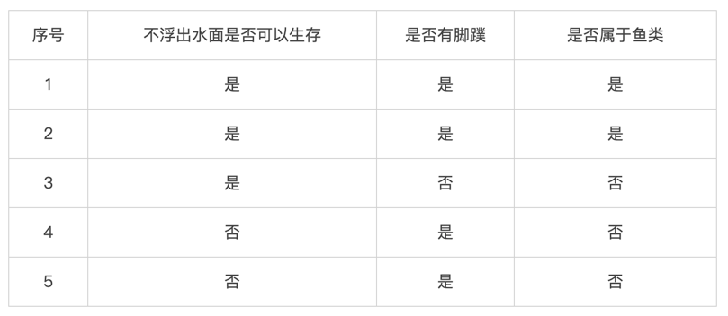<br/> 構成決策樹的原始數據：   <br/> <br/> 接下來算法均采用相同數據集進行考量： <br/> ### 2.3 ID3（Iterative Dichotomiser 3）算法原理 ID3算法的核心是在決策樹各個節點上應用信息增益準則選擇特征遞歸地構建決策樹。 #### 2.3.1 信息增益 **（1） 熵** 在信息論中，熵（entropy）是隨機變量不確定性的度量，也就是熵越大，則隨機變量的不確定性越大。設X是一個取有限個值得離散隨機變量，其概率分布為：  則隨機變量X的熵定義為：  **（2） 條件熵** 設有隨機變量（X, Y），其聯合概率分布為：  條件熵H(Y|X)表示在已知隨機變量X的條件下，隨機變量Y的不確定性。隨機變量X給定的條件下隨機變量Y的條件熵H(Y|X)，定義為X給定條件下Y的條件概率分布的熵對X的數學期望：  當熵和條件熵中的概率由數據估計得到時（如極大似然估計），所對應的熵與條件熵分別稱為經驗熵和經驗條件熵。 **（3）信息增益** **定義：** 信息增益表示由于得知特征A的信息后而使得數據集D的分類不確定性減少的程度，定義為： Gain(D,A) = H(D) – H(D|A) 即集合D的經驗熵H(D)與特征A給定條件下D的經驗條件熵H(H|A)之差。 **理解：** 選擇劃分后信息增益大的作為劃分特征，說明使用該特征后劃分得到的子集純度越高，即不確定性越小。因此我們總是選擇當前使得信息增益最大的特征來劃分數據集。 **缺點：** 信息增益偏向取值較多的特征（原因：當特征的取值較多時，根據此特征劃分更容易得到純度更高的子集，因此劃分后的熵更低，即不確定性更低，因此信息增益更大）<br/> **計算香農熵的代碼實現：** ~~~ def calc_shannon_ent(data_set): """ 計算信息熵 :param data_set: 如： [[1, 1, 'yes'], [1, 1, 'yes'], [1, 0, 'no'], [0, 1, 'no'], [0, 1, 'no']] :return: """ num = len(data_set) # n rows # 為所有的分類類目創建字典 label_counts = {} for feat_vec in data_set: current_label = feat_vec[-1] # 取得最后一列數據 if current_label not in label_counts.keys(): label_counts[current_label] = 0 label_counts[current_label] += 1 # 計算香農熵 shannon_ent = 0.0 for key in label_counts: prob = float(label_counts[key]) / num shannon_ent = shannon_ent - prob * log(prob, 2) return shannon_ent ~~~ * 第一個for循環：為所有可能分類創建字典 * 第二個for循環：以2為底求對數 創建數據集代碼： ~~~ def create_data_set(): """ 創建樣本數據 :return: """ data_set = [[1, 1, 'yes'], [1, 1, 'yes'], [1, 0, 'no'], [0, 1, 'no'], [0, 1, 'no']] labels = ['no surfacing', 'flippers'] return data_set, labels ~~~ 我們分析下熵和混合的數據多少的關系，通過再數據集中添加更多的分類，觀察熵是如何變化的：  > 結論：熵越高，則混合的數據也越多。 #### 2.3.2 ID3算法 ~~~ 輸入：訓練數據集D，特征集A，閾值ε 輸出：決策樹T Step1：若D中所有實例屬于同一類，則T為單結點樹，并將類作為該節點的類標記，返回T； Step2：若A=?，則T為單結點樹，并將D中實例數最大的類作為該節點的類標記，返回T； Step3：否則，計算A中每個特征對D的信息增益，選擇信息增益最大的特征； Step4：如果的信息增益小于閾值ε，則T為單節點樹，并將D中實例數最大的類作為該節點的類標記，返回T Step5：否則，對的每一種可能值，依將D分割為若干非空子集，將中實例數最大的類作為標記，構建子結點，由結點及其子樹構成樹T，返回T； Step6：對第i個子節點，以為訓練集，以為特征集合，遞歸調用Step1~step5，得到子樹，返回； ~~~ #### 2.3.3 代碼實現 ~~~ # -*- coding: utf-8 -*- from math import log import operator import tree_plotter def create_data_set(): """ 創建樣本數據 :return: """ data_set = [[1, 1, 'yes'], [1, 1, 'yes'], [1, 0, 'no'], [0, 1, 'no'], [0, 1, 'no']] labels = ['no surfacing', 'flippers'] return data_set, labels def calc_shannon_ent(data_set): """ 計算信息熵 :param data_set: 如： [[1, 1, 'yes'], [1, 1, 'yes'], [1, 0, 'no'], [0, 1, 'no'], [0, 1, 'no']] :return: """ num = len(data_set) # n rows # 為所有的分類類目創建字典 label_counts = {} for feat_vec in data_set: current_label = feat_vec[-1] # 取得最后一列數據 if current_label not in label_counts.keys(): label_counts[current_label] = 0 label_counts[current_label] += 1 # 計算香濃熵 shannon_ent = 0.0 for key in label_counts: prob = float(label_counts[key]) / num shannon_ent = shannon_ent - prob * log(prob, 2) return shannon_ent def split_data_set(data_set, axis, value): """ 返回特征值等于value的子數據集，切該數據集不包含列（特征）axis :param data_set: 待劃分的數據集 :param axis: 特征索引 :param value: 分類值 :return: """ ret_data_set = [] for feat_vec in data_set: if feat_vec[axis] == value: reduce_feat_vec = feat_vec[:axis] reduce_feat_vec.extend(feat_vec[axis + 1:]) ret_data_set.append(reduce_feat_vec) return ret_data_set def choose_best_feature_to_split(data_set): """ 按照最大信息增益劃分數據 :param data_set: 樣本數據，如： [[1, 1, 'yes'], [1, 1, 'yes'], [1, 0, 'no'], [0, 1, 'no'], [0, 1, 'no']] :return: """ num_feature = len(data_set[0]) - 1 # 特征個數，如：不浮出水面是否可以生存 和是否有腳蹼 base_entropy = calc_shannon_ent(data_set) # 經驗熵H(D) best_info_gain = 0 best_feature_idx = -1 for feature_idx in range(num_feature): feature_val_list = [number[feature_idx] for number in data_set] # 得到某個特征下所有值（某列） unique_feature_val_list = set(feature_val_list) # 獲取無重復的屬性特征值 new_entropy = 0 for feature_val in unique_feature_val_list: sub_data_set = split_data_set(data_set, feature_idx, feature_val) prob = len(sub_data_set) / float(len(data_set)) # 即p(t) new_entropy += prob * calc_shannon_ent(sub_data_set) #對各子集香農熵求和 info_gain = base_entropy - new_entropy # 計算信息增益，g(D,A)=H(D)-H(D|A) # 最大信息增益 if info_gain > best_info_gain: best_info_gain = info_gain best_feature_idx = feature_idx return best_feature_idx def majority_cnt(class_list): """ 統計每個類別出現的次數，并按大到小排序，返回出現次數最大的類別標簽 :param class_list: 類數組 :return: """ class_count = {} for vote in class_list: if vote not in class_count.keys(): class_count[vote] = 0 class_count[vote] += 1 sorted_class_count = sorted(class_count.items(), key=operator.itemgetter(1), reversed=True) print sorted_class_count[0][0] return sorted_class_count[0][0] def create_tree(data_set, labels): """ 構建決策樹 :param data_set: 數據集合，如： [[1, 1, 'yes'], [1, 1, 'yes'], [1, 0, 'no'], [0, 1, 'no'], [0, 1, 'no']] :param labels: 標簽數組，如：['no surfacing', 'flippers'] :return: """ class_list = [sample[-1] for sample in data_set] # ['yes', 'yes', 'no', 'no', 'no'] # 類別相同，停止劃分 if class_list.count(class_list[-1]) == len(class_list): return class_list[-1] # 長度為1，返回出現次數最多的類別 if len(class_list[0]) == 1: return majority_cnt((class_list)) # 按照信息增益最高選取分類特征屬性 best_feature_idx = choose_best_feature_to_split(data_set) # 返回分類的特征的數組索引 best_feat_label = labels[best_feature_idx] # 該特征的label my_tree = {best_feat_label: {}} # 構建樹的字典 del (labels[best_feature_idx]) # 從labels的list中刪除該label，相當于待劃分的子標簽集 feature_values = [example[best_feature_idx] for example in data_set] unique_feature_values = set(feature_values) for feature_value in unique_feature_values: sub_labels = labels[:] # 子集合 # 構建數據的子集合，并進行遞歸 sub_data_set = split_data_set(data_set, best_feature_idx, feature_value) # 待劃分的子數據集 my_tree[best_feat_label][feature_value] = create_tree(sub_data_set, sub_labels) return my_tree def classify(input_tree, feat_labels, test_vec): """ 決策樹分類 :param input_tree: 決策樹 :param feat_labels: 特征標簽 :param test_vec: 測試的數據 :return: """ first_str = list(input_tree.keys())[0] # 獲取樹的第一特征屬性 second_dict = input_tree[first_str] # 樹的分子，子集合Dict feat_index = feat_labels.index(first_str) # 獲取決策樹第一層在feat_labels中的位置 for key in second_dict.keys(): if test_vec[feat_index] == key: if type(second_dict[key]).__name__ == 'dict': class_label = classify(second_dict[key], feat_labels, test_vec) else: class_label = second_dict[key] return class_label 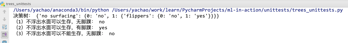data_set, labels = create_data_set() decision_tree = create_tree(data_set, labels) print "決策樹：", decision_tree data_set, labels = create_data_set() print "（1）不浮出水面可以生存，無腳蹼：", classify(decision_tree, labels, [1, 0]) print "（2）不浮出水面可以生存，有腳蹼：", classify(decision_tree, labels, [1, 1]) print "（3）不浮出水面可以不能生存，無腳蹼：", classify(decision_tree, labels, [0, 0]) 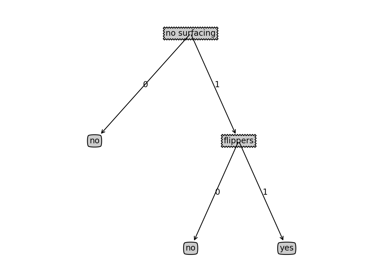tree_plotter.create_plot(decision_tree) ~~~ 畫圖程序 tree_plotter.py： ~~~ import matplotlib.pyplot as plt decision_node = dict(boxstyle="sawtooth", fc="0.8") leaf_node = dict(boxstyle="round4", fc="0.8") arrow_args = dict(arrowstyle="<-") def plot_node(node_txt, center_pt, parent_pt, node_type): create_plot.ax1.annotate(node_txt, xy=parent_pt, xycoords='axes fraction', \ xytext=center_pt, textcoords='axes fraction', \ va="center", ha="center", bbox=node_type, arrowprops=arrow_args) def get_num_leafs(my_tree): num_leafs = 0 first_str = list(my_tree.keys())[0] second_dict = my_tree[first_str] for key in second_dict.keys(): if type(second_dict[key]).__name__ == 'dict': num_leafs += get_num_leafs(second_dict[key]) else: num_leafs += 1 return num_leafs def get_tree_depth(my_tree): max_depth = 0 first_str = list(my_tree.keys())[0] second_dict = my_tree[first_str] for key in second_dict.keys(): if type(second_dict[key]).__name__ == 'dict': thisDepth = get_tree_depth(second_dict[key]) + 1 else: thisDepth = 1 if thisDepth > max_depth: max_depth = thisDepth return max_depth def plot_mid_text(cntr_pt, parent_pt, txt_string): x_mid = (parent_pt[0] - cntr_pt[0]) / 2.0 + cntr_pt[0] y_mid = (parent_pt[1] - cntr_pt[1]) / 2.0 + cntr_pt[1] create_plot.ax1.text(x_mid, y_mid, txt_string) def plot_tree(my_tree, parent_pt, node_txt): num_leafs = get_num_leafs(my_tree) depth = get_tree_depth(my_tree) first_str = list(my_tree.keys())[0] cntr_pt = (plot_tree.x_off + (1.0 + float(num_leafs)) / 2.0 / plot_tree.total_w, plot_tree.y_off) plot_mid_text(cntr_pt, parent_pt, node_txt) plot_node(first_str, cntr_pt, parent_pt, decision_node) second_dict = my_tree[first_str] plot_tree.y_off = plot_tree.y_off - 1.0 / plot_tree.total_d for key in second_dict.keys(): if type(second_dict[key]).__name__ == 'dict': plot_tree(second_dict[key], cntr_pt, str(key)) else: plot_tree.x_off = plot_tree.x_off + 1.0 / plot_tree.total_w plot_node(second_dict[key], (plot_tree.x_off, plot_tree.y_off), cntr_pt, leaf_node) plot_mid_text((plot_tree.x_off, plot_tree.y_off), cntr_pt, str(key)) plot_tree.y_off = plot_tree.y_off + 1.0 / plot_tree.total_d def create_plot(in_tree): fig = plt.figure(1, facecolor='white') fig.clf() axprops = dict(xticks=[], yticks=[]) create_plot.ax1 = plt.subplot(111, frameon=False, **axprops) plot_tree.total_w = float(get_num_leafs(in_tree)) plot_tree.total_d = float(get_tree_depth(in_tree)) plot_tree.x_off = -0.5 / plot_tree.total_w plot_tree.y_off = 1.0 plot_tree(in_tree, (0.5, 1.0), '') plt.show() ~~~ 運行結果：   ### 2.4 C4.5算法原理 C4.5算法與ID3算法很相似，C4.5算法是對ID3算法做了改進，在生成決策樹過程中采用信息增益比來選擇特征。 #### 2.4.1信息增益比 我們知道信息增益會偏向取值較多的特征，使用信息增益比可以對這一問題進行校正。 **定義**：特征A對訓練數據集D的信息增益比GainRatio(D,A)定義為其信息增益Gain(D,A)與訓練數據集D的經驗熵H(D)之比：  #### 2.4.2 C4.5算法 C4.5算法過程跟ID3算法一樣，只是選擇特征的方法由信息增益改成信息增益比。 具體過程，同2.3.2 #### 2.4.3 代碼實現 我們還是采用2.1.3中的實例，C4.5算法跟ID3算法，不同的地方只是特征選擇方法，即調整特征選擇方法代碼即可： ~~~ def choose_best_feature_to_split(data_set): """ 按照最大信息增益比劃分數據 :param data_set: 樣本數據，如： [[1, 1, 'yes'], [1, 1, 'yes'], [1, 0, 'no'], [0, 1, 'no'], [0, 1, 'no']] :return: """ num_feature = len(data_set[0]) - 1 # 特征個數，如：不浮出水面是否可以生存 和是否有腳蹼 base_entropy = calc_shannon_ent(data_set) # 經驗熵H(D) best_info_gain_ratio = 0.0 best_feature_idx = -1 for feature_idx in range(num_feature): # 得到某個特征下所有值（某列） feature_val_list = [number[feature_idx] for number in data_set] # 獲取無重復的屬性特征值 unique_feature_val_list = set(feature_val_list) new_entropy = 0 split_info = 0.0 for value in unique_feature_val_list: sub_data_set = split_data_set(data_set, feature_idx, value) # 即p(t) prob = len(sub_data_set) / float(len(data_set)) # 對各子集香農熵求和 new_entropy += prob * calc_shannon_ent(sub_data_set) split_info += -prob * log(prob, 2) # 計算信息增益，g(D,A)=H(D)-H(D|A) info_gain = base_entropy - new_entropy if split_info == 0: # fix the overflow bug continue info_gain_ratio = info_gain / split_info # 最大信息增益比 if info_gain_ratio > best_info_gain_ratio: best_info_gain_ratio = info_gain_ratio best_feature_idx = feature_idx return best_feature_idx ~~~ ### 2.5 CART算法原理 > CART樹里面對C4.5中存在的問題進行了改進。CART假設決策樹是二叉樹，并且可以分類也可以回歸，而且用基尼指數代替了熵模型進行特征選擇，也提供了優化的剪枝策略。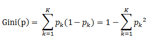 #### 2.5.1 Gini指數 分類問題中，假設有K個類，樣本點屬于第k類的概率為，則概率分布的基尼指數定義為：  備注：表示選中的樣本屬于k類別的概率，則這個樣本被分錯的概率為 對于給定的樣本集合D，其基尼指數為：  備注：這里是D中屬于第k類的樣本自己，K是類的個數。 如果樣本集合D根據特征A是否取某一可能值a被分割成D1和D2兩部分，即：  則在特征A的條件下，集合D的基尼指數定義為：  基尼指數Gini(D)表示集合D的不確定性，基尼指數Gini(D,A)表示經A=a分割后集合D的不確定性。基尼指數值越大，樣本集合的不確定性也就越大，這一點跟熵相似。 <strong style="color:green;">[看例子解讀]</strong> 如下，是一個包含30個學生的樣本，其包含三種特征，分別是：性別（男/女）、班級（IX/X）和高度（5到6ft）。其中30個學生里面有15個學生喜歡在閑暇時間玩板球。那么要如何選擇第一個要劃分的特征呢，我們通過上面的公式來進行計算。  如下，可以Gini(D,Gender)最小，所以選擇性別作為最優特征。  #### 2.5.2 CART算法 ~~~ 輸入：訓練數據集D，停止計算的條件 輸出：CART決策樹 根據訓練數據集，從根結點開始，遞歸地對每個結點進行以下操作，構建二叉樹： Step1：設結點的訓練數據集為D，計算現有特征對該數據集的基尼指數。此時，對每一個特征A，對其可能取的每個值a，根據樣本點A=a的測試為“是”或“否”將D分割為D1和D2兩部分，利用上式Gini(D,A)來計算A=a時的基尼指數。 Step2：在所有可能的特征A以及他們所有可能的切分點a中，選擇基尼指數最小的特征及其對應可能的切分點作為最有特征與最優切分點。依最優特征與最有切分點，從現結點生成兩個子節點，將訓練數據集依特征分配到兩個子節點中去。 Step3：對兩個子結點遞歸地調用Step1、Step2，直至滿足條件。 Step4：生成CART決策樹 算法停止計算的條件是節點中的樣本個數小于預定閾值，或樣本集的基尼指數小于預定閾值，或者沒有更多特征。 ~~~ #### 2.5.4 代碼實現 ~~~ # -*- coding: utf-8 -*- import numpy as np class Tree(object): def __init__(self, value=None, true_branch=None, false_branch=None, results=None, col=-1, summary=None, data=None): self.value = value self.true_branch = true_branch self.false_branch = false_branch self.results = results self.col = col self.summary = summary self.data = data def __str__(self): print(self.col, self.value) print(self.results) print(self.summary) return "" def split_datas(rows, value, column): """ 根據條件分離數據集 :param rows: :param value: :param column: :return: (list1, list2) """ list1 = [] list2 = [] if isinstance(value, int) or isinstance(value, float): for row in rows: if row[column] >= value: list1.append(row) else: list2.append(row) else: for row in rows: if row[column] == value: list1.append(row) else: list2.append(row) return list1, list2 def calculate_diff_count(data_set): """ 分類統計data_set中每個類別的數量 :param datas:如：[[5.1, 3.5, 1.4, 0.2, 'setosa'], [4.9, 3, 1.4, 0.2, 'setosa'],....] :return: 如：{'setosa': 50, 'versicolor': 50, 'virginica': 50} """ results = {} for data in data_set: # 數據的最后一列data[-1]是類別 if data[-1] not in results: results.setdefault(data[-1], 1) else: results[data[-1]] += 1 return results def gini(data_set): """ 計算gini的值，即Gini(p) :param data_set: 如：[[5.1, 3.5, 1.4, 0.2, 'setosa'], [4.9, 3, 1.4, 0.2, 'setosa'],....] :return: """ length = len(data_set) category_2_cnt = calculate_diff_count(data_set) sum = 0.0 for category in category_2_cnt: sum += pow(float(category_2_cnt[category]) / length, 2) return 1 - sum def build_decision_tree(data_set, evaluation_function=gini): """ 遞歸建立決策樹，當gain=0時，停止回歸 :param data_set: 如：[[5.1, 3.5, 1.4, 0.2, 'setosa'], [4.9, 3, 1.4, 0.2, 'setosa'],....] :param evaluation_function: :return: """ current_gain = evaluation_function(data_set) column_length = len(data_set[0]) rows_length = len(data_set) best_gain = 0.0 best_value = None best_set = None # choose the best gain for feature_idx in range(column_length - 1): feature_value_set = set(row[feature_idx] for row in data_set) for feature_value in feature_value_set: sub_data_set1, sub_data_set2 = split_datas(data_set, feature_value, feature_idx) p = float(len(sub_data_set1)) / rows_length # Gini(D,A)表示在特征A的條件下集合D的基尼指數，gini_d_a越小，樣本集合不確定性越小 # 我們的目的是找到另gini_d_a最小的特征，及gain最大的特征 gini_d_a = p * evaluation_function(sub_data_set1) + (1 - p) * evaluation_function(sub_data_set2) gain = current_gain - gini_d_a if gain > best_gain: best_gain = gain best_value = (feature_idx, feature_value) best_set = (sub_data_set1, sub_data_set2) dc_y = {'impurity': '%.3f' % current_gain, 'sample': '%d' % rows_length} # stop or not stop if best_gain > 0: true_branch = build_decision_tree(best_set[0], evaluation_function) false_branch = build_decision_tree(best_set[1], evaluation_function) return Tree(col=best_value[0], value=best_value[1], true_branch=true_branch, false_branch=false_branch, summary=dc_y) else: return Tree(results=calculate_diff_count(data_set), summary=dc_y, data=data_set) def prune(tree, mini_gain, evaluation_function=gini): """ 裁剪 :param tree: :param mini_gain: :param evaluation_function: :return: """ if tree.true_branch.results == None: prune(tree.true_branch, mini_gain, evaluation_function) if tree.false_branch.results == None: prune(tree.false_branch, mini_gain, evaluation_function) if tree.true_branch.results != None and tree.false_branch.results != None: len1 = len(tree.true_branch.data) len2 = len(tree.false_branch.data) len3 = len(tree.true_branch.data + tree.false_branch.data) p = float(len1) / (len1 + len2) gain = evaluation_function(tree.true_branch.data + tree.false_branch.data) \ - p * evaluation_function(tree.true_branch.data)\ - (1 - p) * evaluation_function(tree.false_branch.data) if gain < mini_gain: # 當節點的gain小于給定的 mini Gain時則合并這兩個節點 tree.data = tree.true_branch.data + tree.false_branch.data tree.results = calculate_diff_count(tree.data) tree.true_branch = None tree.false_branch = None def classify(data, tree): """ 分類 :param data: :param tree: :return: """ if tree.results != None: return tree.results else: branch = None v = data[tree.col] if isinstance(v, int) or isinstance(v, float): if v >= tree.value: branch = tree.true_branch else: branch = tree.false_branch else: if v == tree.value: branch = tree.true_branch else: branch = tree.false_branch return classify(data, branch) def load_csv(): def convert_types(s): s = s.strip() try: return float(s) if '.' in s else int(s) except ValueError: return s data = np.loadtxt("datas.csv", dtype="str", delimiter=",") data = data[1:, :] data_set = ([[convert_types(item) for item in row] for row in data]) return data_set ~~~ <br/> ## 2.6何時選擇決策樹算法？？？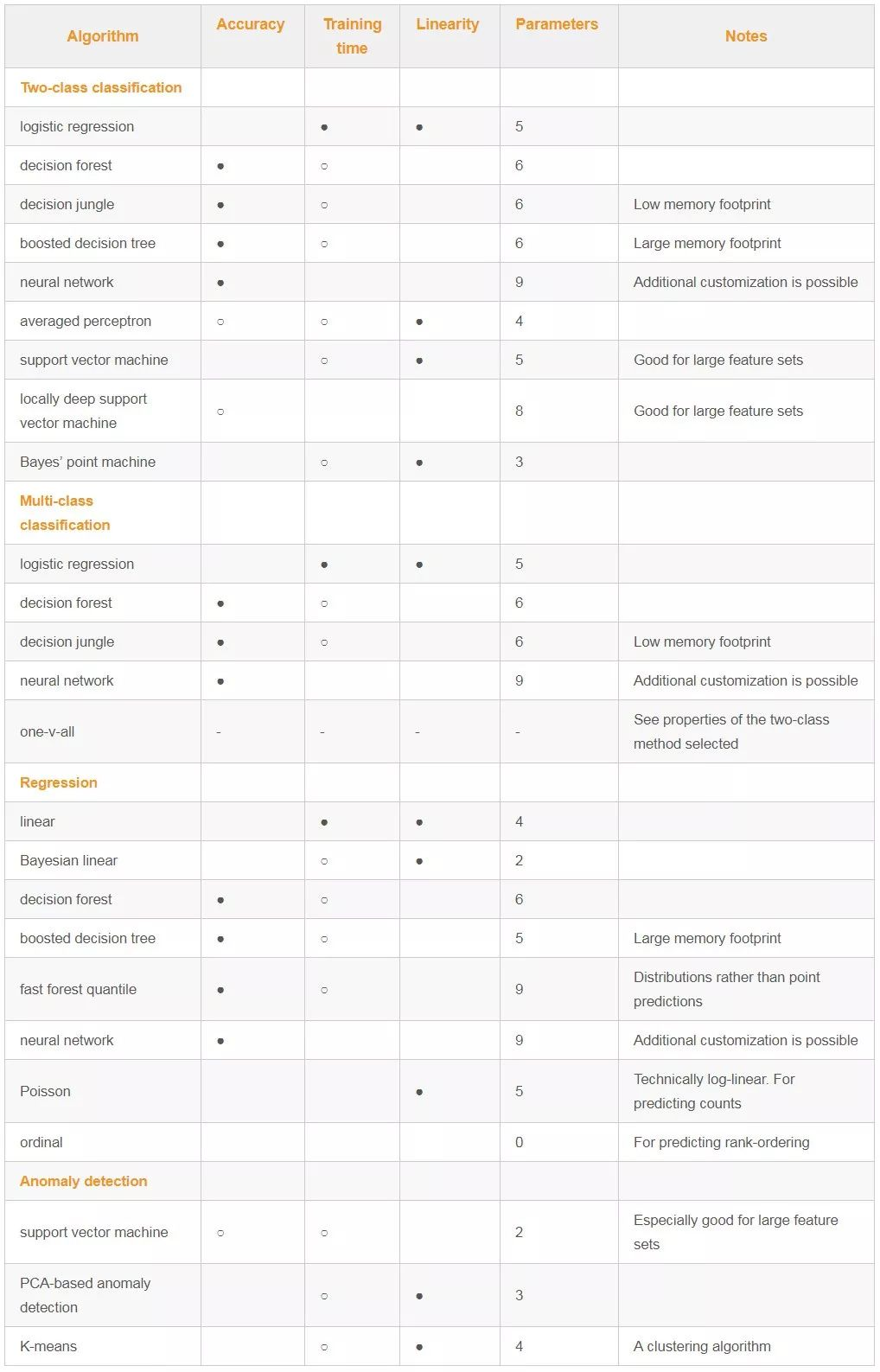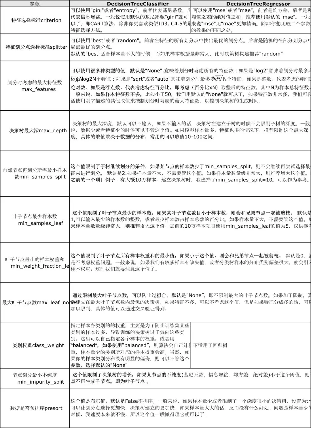 scikit-learn決策樹使用指南：[https://scikit-learn.org/dev/modules/classes.html#module-sklearn.tree](https://scikit-learn.org/dev/modules/classes.html#module-sklearn.tree) 參數說明： <br/> 何時選擇決策樹算法？：  ## 3.總結 * ID3 * 局限性 * （1）不支持連續特征 * （2）采用信息增益大的特征優先建立決策樹的節點。在相同條件下，取值比較多的特征比取值少的特征信息增益大。 * （3）不支持缺失值處理 * （4）沒有應對過擬合的策略 * C4.5 * 局限性 * （1）剪枝的算法有非常多，C4.5的剪枝方法有優化的空間 * （2）C4.5生成的是多叉樹，很多時候，在計算機中二叉樹模型會比多叉樹運算效率高。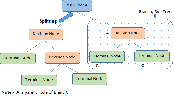如果采用二叉樹，可以提高效率 * （3）C4.5只能用于分類 * （4）C4.5使用了熵模型，里面有大量的耗時的對數運算,如果是連續值還有大量的排序運算 * CART ## <strong>附錄一：決策樹相關的重要概念</strong> （1）根結點(Root Node)：它表示整個樣本集合，并且該節點可以進一步劃分成兩個或多個子集。 （2）拆分(Splitting)：表示將一個結點拆分成多個子集的過程。 （3）決策結點(Decision Node)：當一個子結點進一步被拆分成多個子節點時，這個子節點就叫做決策結點。 （4）葉子結點(Leaf/Terminal Node)：無法再拆分的結點被稱為葉子結點。 （5）剪枝(Pruning)：移除決策樹中子結點的過程就叫做剪枝，跟拆分過程相反。 （6）分支/子樹(Branch/Sub-Tree)：一棵決策樹的一部分就叫做分支或子樹。 （7）父結點和子結點(Paren and Child Node)：一個結點被拆分成多個子節點，這個結點就叫做父節點；其拆分后的子結點也叫做子結點。  ## <strong>附錄二：參考資料</strong> * [決策樹算法原理(上)](https://www.cnblogs.com/pinard/p/6050306.html) * [決策樹算法的原理（接地氣版）](https://my.oschina.net/u/3658210/blog/4526316) * [決策樹例題](https://wenku.baidu.com/view/6eb1c1df1fd9ad51f01dc281e53a580217fc5011.html ) * [帶你搞懂決策樹算法原理](https://blog.csdn.net/akirameiao/article/details/79953980) * [python機器學習筆記：深入學習決策樹算法原理](https://www.cnblogs.com/wj-1314/p/9428494.html) * [跟我一起學scikit-learn18：決策樹算法](https://blog.csdn.net/u011436316/article/details/92141250) * [為什么在神經網絡大放異彩的今天要學習決策樹？](https://www.zhihu.com/question/54811425?sort=created) * [Python機器學習算法庫scikit-learn學習之決策樹實現方法詳解](https://www.jb51.net/article/164614.htm) * 書籍推薦：[機器學習實戰：基于Scikit-Learn和TensorFlow PDF下載](http://www.java1234.com/a/javabook/javabase/2018/1128/12462.html) ## <strong>附錄三：算法比較圖</strong>