# 第三部分 聚類
## 三十四、聚類簡介
歡迎閱讀第三十四篇教程。這篇教程是聚類和非監督機器學習的開始。到現在為止,每個我們涉及到的東西都是“監督”機器學習,也就是說,我們科學家,告訴機器特征集有什么分類。但是在非監督機器學習下,科學家的角色就溢出了。首先,我們會涉及聚類,它有兩種形式,扁平和層次化的。
對于這兩種形式的聚類,機器的任務是,接受僅僅是特征集的數據集,之后搜索分組并分配標簽。對于扁平化聚類,科學家告訴機器要尋找多少個分類或簇。對于層次化聚類,機器會自己尋找分組及其數量。
我們為什么要利用聚類呢?聚類的目標就是尋找數據中的關系和含義。多數情況下,我自己看到了,人們將聚類用于所謂的“半監督”機器學習。這里的想法是,你可以使用聚類來定義分類。另一個用途就是特征選取和驗證。例如,考慮我們的乳腺腫瘤數據集。我們可能認為,我們選取的特征缺失是描述性并且有意義的。我們擁有的一個選項,就是將數據扔給 KMeans 算法,之后觀察數據實際上是否描述了我們跟蹤的兩個分組,以我們預期的方式。
下面假設,你是個 Amazon 的樹科學家。你的 CTO 收集了數據,并且認為可以用于預測顧客是不是買家。它們希望你使用 KMeans 來看看是否 KMeans 正確按照數據來組織用戶,CTO 認為這個很有意義。
層次聚類是什么?假設你仍然是那個相同的數據科學家。這一次,你使用層次聚類算法處理看似有意義的數據,例如均值漂移,并且實際上獲取了五個分組。在深入分析之后,你意識到訪問者實際上不是買家或者非買家,它們實際上是個光譜。實際上有非買家、可能的非買家、低可能的買家、高可能的馬甲,和確定的買家。
聚類也可以用于真正的未知數據,來嘗試尋找結構。假設你是個探索北美人類文字的外星人。你可能收集了所有手寫字符,將其編譯為一個大型的特征列表。之后你可能將這個列表扔給層次聚類算法,來看看是否可以尋找特定的分組,以便通過字符解碼語言。
“大數據分析”的領域通常是聚類的初始區域。這里有大量的數據,但是如何處理他們,或者如何獲取他們的含義,多數公司完全沒有概念。聚類可以幫助數據科學家,來分析大量數據集的結構,以及尋找它們的含義。
最后,聚類也可以用于典型的分類,你實際上并不需要將其扔給分類算法,但是如果你在多數主流的分類數據集上使用聚類,你應該能發現,它能夠找到分組。
我們第一個算法是 KMeans。KMeans 的思路就是嘗試將給定數據集聚類到 K 個簇中。它的工作方式令人印象深刻。并且我們足夠幸運,他還非常簡單。這個過程是:
1. 獲取真個數據集,并隨機設置 K 個形心。形心就是簇的“中心”。首先,我通常選取前 K 個值,并使用它們來開始,但是你也可以隨機選取它們。這應該沒關系,但是,如果你不為了一些原因做優化,可能就需要嘗試打亂數據并再次嘗試。
2. 計算每個數據集到形心的距離,1并按照形心的接近程度來分類每個數據集。形心的分類是任意的,你可能將第一個形心命名為 0,第二個為 1,以此類推。
3. 一旦已經分類好了數據,現在計算分組的均值,并將均值設為新的形心。
4. 重復第二和第三步直到最優。通常,你通過形心的移動來度量優化。有很多方式來這么做,我們僅僅使用百分數比例。
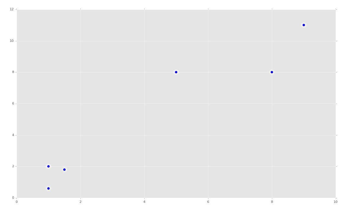
很簡單,比 SVM 簡單多了。讓我們看看一個簡短的代碼示例。開始,我們擁有這樣一些數據:
```py
import matplotlib.pyplot as plt
from matplotlib import style
import numpy as np
from sklearn.cluster import KMeans
style.use('ggplot')
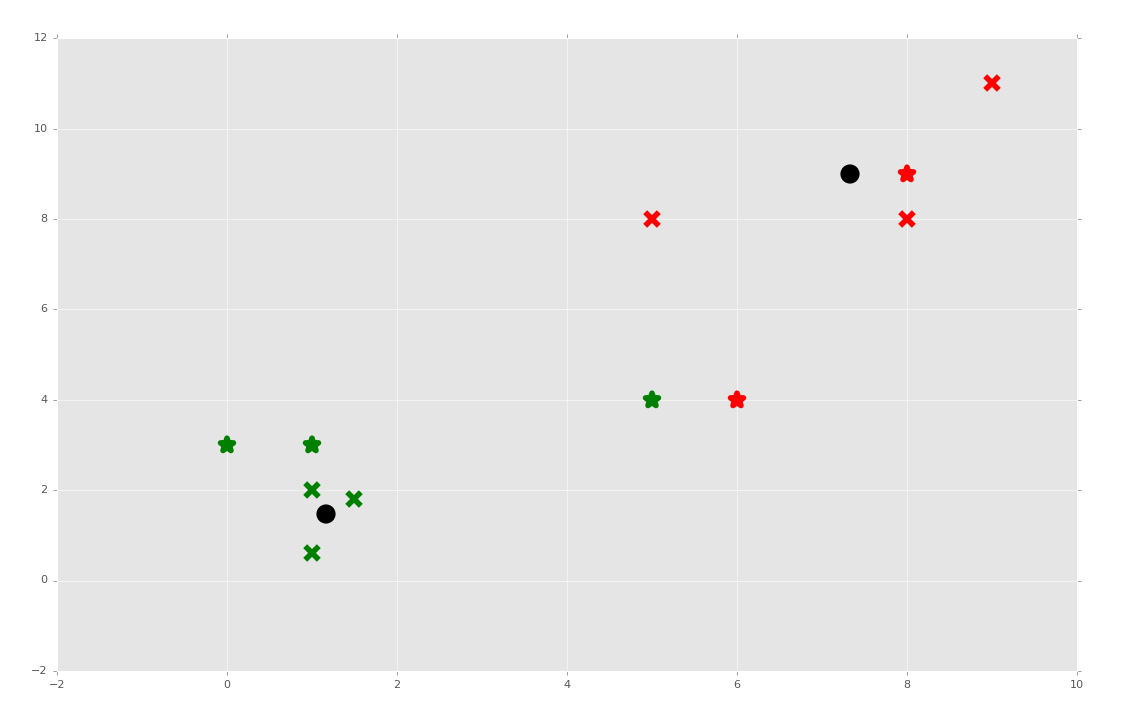
#ORIGINAL:
X = np.array([[1, 2],
[1.5, 1.8],
[5, 8],
[8, 8],
[1, 0.6],
[9, 11]])
plt.scatter(X[:, 0],X[:, 1], s=150, linewidths = 5, zorder = 10)
plt.show()
```
我們的數據是:
太棒了,看起來很簡單,所以我們的 KMeans 算法更適于這個東西。首先我們會嘗試擬合所有東西:
```py
clf = KMeans(n_clusters=2)
clf.fit(X)
```
就這么簡單,但是我們可能希望看到它。我們之前在 SVM 中看到過,多數 Sklearn 分類器都擁有多種屬性。使用 KMeans 算法,我們可以獲取形心和標簽。
```py
centroids = clf.cluster_centers_
labels = clf.labels_
```
現在繪制他們:
```py
colors = ["g.","r.","c.","y."]
for i in range(len(X)):
plt.plot(X[i][0], X[i][1], colors[labels[i]], markersize = 10)
plt.scatter(centroids[:, 0],centroids[:, 1], marker = "x", s=150, linewidths = 5, zorder = 10)
plt.show()
```
下面,我們打算講 KMeans 算法應用于真實的數據集,并且涉及,如果你的數據含有非數值的信息,會發生什么。
## 三十五、處理非數值數據
歡迎閱讀第三十五篇教程。我們最近開始談論聚類,但是這個教程中,我們打算涉及到處理非數值數據,它當然不是聚類特定的。
我們打算處理的數據是[泰坦尼克數據集](https://pythonprogramming.net/static/downloads/machine-learning-data/titanic.xls)。
簡單看一下數據和值:
```
Pclass Passenger Class (1 = 1st; 2 = 2nd; 3 = 3rd)
survival Survival (0 = No; 1 = Yes)
name Name
sex Sex
age Age
sibsp Number of Siblings/Spouses Aboard
parch Number of Parents/Children Aboard
ticket Ticket Number
fare Passenger Fare (British pound)
cabin Cabin
embarked Port of Embarkation (C = Cherbourg; Q = Queenstown; S = Southampton)
boat Lifeboat
body Body Identification Number
home.dest Home/Destination
```
這個數據集的主要關注點就是`survival `一列。在使用監督式機器學習的時候,你要將這一列看做分類,對其訓練數據。但是對于聚類,我們讓機器生產分組,并自行貼標簽。我的第一個興趣點事,是否分組和任何列相關,尤其是`survival `一列。對于我們這個教程,我們現在執行扁平聚類,也就是我們告訴機器想要兩個分組,但是之后我們也會讓機器決定分組數量。
但是現在,我們要面對另一個問題。如果我們將這個數據加載進 Pandas,我們會看到這樣一些東西:
```py
#https://pythonprogramming.net/static/downloads/machine-learning-data/titanic.xls
import matplotlib.pyplot as plt
from matplotlib import style
style.use('ggplot')
import numpy as np
from sklearn.cluster import KMeans
from sklearn import preprocessing, cross_validation
import pandas as pd
'''
Pclass Passenger Class (1 = 1st; 2 = 2nd; 3 = 3rd)
survival Survival (0 = No; 1 = Yes)
name Name
sex Sex
age Age
sibsp Number of Siblings/Spouses Aboard
parch Number of Parents/Children Aboard
ticket Ticket Number
fare Passenger Fare (British pound)
cabin Cabin
embarked Port of Embarkation (C = Cherbourg; Q = Queenstown; S = Southampton)
boat Lifeboat
body Body Identification Number
home.dest Home/Destination
'''
df = pd.read_excel('titanic.xls')
print(df.head())
```
```
pclass survived name sex \
0 1 1 Allen, Miss. Elisabeth Walton female
1 1 1 Allison, Master. Hudson Trevor male
2 1 0 Allison, Miss. Helen Loraine female
3 1 0 Allison, Mr. Hudson Joshua Creighton male
4 1 0 Allison, Mrs. Hudson J C (Bessie Waldo Daniels) female
age sibsp parch ticket fare cabin embarked boat body \
0 29.0000 0 0 24160 211.3375 B5 S 2 NaN
1 0.9167 1 2 113781 151.5500 C22 C26 S 11 NaN
2 2.0000 1 2 113781 151.5500 C22 C26 S NaN NaN
3 30.0000 1 2 113781 151.5500 C22 C26 S NaN 135.0
4 25.0000 1 2 113781 151.5500 C22 C26 S NaN NaN
home.dest
0 St Louis, MO
1 Montreal, PQ / Chesterville, ON
2 Montreal, PQ / Chesterville, ON
3 Montreal, PQ / Chesterville, ON
4 Montreal, PQ / Chesterville, ON
pclass survived name sex age sibsp parch ticket fare \
0 1 1 110 0 29.0000 0 0 748 211.3375
1 1 1 839 1 0.9167 1 2 504 151.5500
2 1 0 1274 0 2.0000 1 2 504 151.5500
3 1 0 284 1 30.0000 1 2 504 151.5500
4 1 0 563 0 25.0000 1 2 504 151.5500
cabin embarked boat body home.dest
0 52 1 1 NaN 173
1 44 1 6 NaN 277
2 44 1 0 NaN 277
3 44 1 0 135.0 277
4 44 1 0 NaN 277
```
問題是,我們得到了非數值的數據。機器學習算法需要數值。我們可以丟棄`name`列,它對我們沒有用。我們是否應該丟棄`sex`列呢?我不這么看,它看起來是特別重要的列,尤其是我們知道“女士和孩子是有限的”。那么`cabin`列又如何呢?可能它對于你在船上的位置很重要呢?我猜是這樣。可能你從哪里乘船不是很重要,但是這個時候,我們已經知道了我們需要以任何方式處理非數值數據。
有很多方式處理非數值數據,這就是我自己使用的方式。首先,你打算遍歷 Pandas 數據幀中的列。對于不是數值的列,你想要尋找它們的唯一元素。這可以簡單通過獲取列值的`set`來完成。這里,`set`中的索引也可以是新的“數值”值,或者文本數據的“id”。
開始:
```py
def handle_non_numerical_data(df):
columns = df.columns.values
for column in columns:
```
創建函數,獲取列,迭代它們。繼續:
```py
def handle_non_numerical_data(df):
columns = df.columns.values
for column in columns:
text_digit_vals = {}
def convert_to_int(val):
return text_digit_vals[val]
if df[column].dtype != np.int64 and df[column].dtype != np.float64:
column_contents = df[column].values.tolist()
unique_elements = set(column_contents)
```
這里,我們添加了嵌套函數,將參數值作為鍵,轉換為這個元素在`text_digit_vals`中的值。我們現在還不使用它,但是也快了。下面,當我們迭代列的時候,我們打算確認是否這一列是`np.int64`或`np.float64`。如果不是,我們將這一列轉換為值的列表,之后我們獲取這一列的`set`來獲取唯一的值。
```py
def handle_non_numerical_data(df):
columns = df.columns.values
for column in columns:
text_digit_vals = {}
def convert_to_int(val):
return text_digit_vals[val]
if df[column].dtype != np.int64 and df[column].dtype != np.float64:
column_contents = df[column].values.tolist()
unique_elements = set(column_contents)
x = 0
for unique in unique_elements:
if unique not in text_digit_vals:
text_digit_vals[unique] = x
x+=1
df[column] = list(map(convert_to_int, df[column]))
return df
```
我們繼續,對于每個找到的唯一元素,我們創建新的字典,鍵是唯一元素,值是新的數值。一旦我們迭代了所有的唯一元素,我們就將之前創建的函數映射到這一列上。不知道什么是映射嘛?查看[這里](https://pythonprogramming.net/rolling-apply-mapping-functions-data-analysis-python-pandas-tutorial/)。
現在我們添加一些代碼:
```py
df = handle_non_numerical_data(df)
print(df.head())
```
完整代碼:
```py
#https://pythonprogramming.net/static/downloads/machine-learning-data/titanic.xls
import matplotlib.pyplot as plt
from matplotlib import style
style.use('ggplot')
import numpy as np
from sklearn.cluster import KMeans
from sklearn import preprocessing, cross_validation
import pandas as pd
'''
Pclass Passenger Class (1 = 1st; 2 = 2nd; 3 = 3rd)
survival Survival (0 = No; 1 = Yes)
name Name
sex Sex
age Age
sibsp Number of Siblings/Spouses Aboard
parch Number of Parents/Children Aboard
ticket Ticket Number
fare Passenger Fare (British pound)
cabin Cabin
embarked Port of Embarkation (C = Cherbourg; Q = Queenstown; S = Southampton)
boat Lifeboat
body Body Identification Number
home.dest Home/Destination
'''
df = pd.read_excel('titanic.xls')
#print(df.head())
df.drop(['body','name'], 1, inplace=True)
df.convert_objects(convert_numeric=True)
df.fillna(0, inplace=True)
#print(df.head())
def handle_non_numerical_data(df):
columns = df.columns.values
for column in columns:
text_digit_vals = {}
def convert_to_int(val):
return text_digit_vals[val]
if df[column].dtype != np.int64 and df[column].dtype != np.float64:
column_contents = df[column].values.tolist()
unique_elements = set(column_contents)
x = 0
for unique in unique_elements:
if unique not in text_digit_vals:
text_digit_vals[unique] = x
x+=1
df[column] = list(map(convert_to_int, df[column]))
return df
df = handle_non_numerical_data(df)
print(df.head())
```
輸出:
```
pclass survived sex age sibsp parch ticket fare cabin \
0 1 1 1 29.0000 0 0 767 211.3375 80
1 1 1 0 0.9167 1 2 531 151.5500 149
2 1 0 1 2.0000 1 2 531 151.5500 149
3 1 0 0 30.0000 1 2 531 151.5500 149
4 1 0 1 25.0000 1 2 531 151.5500 149
embarked boat home.dest
0 1 1 307
1 1 27 43
2 1 0 43
3 1 0 43
4 1 0 43
```
如果`df.convert_objects(convert_numeric=True)`出現了廢棄警告,或者錯誤,盡管將其注釋掉吧。我通常為了清楚而保留它,但是數據幀應該把數值讀作數值。出于一些原因,Pandas 會隨機將列中的一些行讀作字符串,盡管字符串實際上是數值。對我來說沒有意義,所以我將將它們轉為字符串來保證。
太好了,所以我們得到了數值,現在我們可以繼續使用這個數據做扁平聚類了。
## 三十六、泰坦尼克數據集 KMeans
歡迎閱讀第三十六篇教程,另一篇話題為聚類的教程。
之前的教程中,我們涉及了如何處理非數值的數據,這里我們打算實際對泰坦尼克數據集應用 KMeans 算法。KMeans 算法是個扁平聚類算法,也就是說我們需要告訴機器一件事情,應該有多少個簇。我們打算告訴算法有兩個分組,之后我們讓機器尋找幸存者和遇難者,基于它選取的這兩個分組。
我們的代碼為:
```py
#https://pythonprogramming.net/static/downloads/machine-learning-data/titanic.xls
import matplotlib.pyplot as plt
from matplotlib import style
style.use('ggplot')
import numpy as np
from sklearn.cluster import KMeans
from sklearn import preprocessing
import pandas as pd
'''
Pclass Passenger Class (1 = 1st; 2 = 2nd; 3 = 3rd)
survival Survival (0 = No; 1 = Yes)
name Name
sex Sex
age Age
sibsp Number of Siblings/Spouses Aboard
parch Number of Parents/Children Aboard
ticket Ticket Number
fare Passenger Fare (British pound)
cabin Cabin
embarked Port of Embarkation (C = Cherbourg; Q = Queenstown; S = Southampton)
boat Lifeboat
body Body Identification Number
home.dest Home/Destination
'''
df = pd.read_excel('titanic.xls')
#print(df.head())
df.drop(['body','name'], 1, inplace=True)
df.convert_objects(convert_numeric=True)
df.fillna(0, inplace=True)
#print(df.head())
def handle_non_numerical_data(df):
columns = df.columns.values
for column in columns:
text_digit_vals = {}
def convert_to_int(val):
return text_digit_vals[val]
if df[column].dtype != np.int64 and df[column].dtype != np.float64:
column_contents = df[column].values.tolist()
unique_elements = set(column_contents)
x = 0
for unique in unique_elements:
if unique not in text_digit_vals:
text_digit_vals[unique] = x
x+=1
df[column] = list(map(convert_to_int, df[column]))
return df
df = handle_non_numerical_data(df)
```
這里,我們可以立即執行聚類:
```py
X = np.array(df.drop(['survived'], 1).astype(float))
y = np.array(df['survived'])
clf = KMeans(n_clusters=2)
clf.fit(X)
```
好的,現在讓我們看看,是否分組互相匹配。你可以注意,這里,幸存者是 0,遇難者是 1。對于聚類算法,機器會尋找簇,但是會給簇分配任意標簽,以便尋找它們。因此,幸存者的分組可能是 0 或者 1,取決于隨機度。因此,如果你的一致性是 30% 或者 70%,那么你的模型準確度是 70%。讓我們看看吧:
```py
correct = 0
for i in range(len(X)):
predict_me = np.array(X[i].astype(float))
predict_me = predict_me.reshape(-1, len(predict_me))
prediction = clf.predict(predict_me)
if prediction[0] == y[i]:
correct += 1
print(correct/len(X))
# 0.4957983193277311
```
準確度是 49% ~ 51%,不是很好。還記得幾篇教程之前,預處理的事情嗎?當我們之前使用的時候,看起來不是很重要,但是這里呢?
```py
X = np.array(df.drop(['survived'], 1).astype(float))
X = preprocessing.scale(X)
y = np.array(df['survived'])
clf = KMeans(n_clusters=2)
clf.fit(X)
correct = 0
for i in range(len(X)):
predict_me = np.array(X[i].astype(float))
predict_me = predict_me.reshape(-1, len(predict_me))
prediction = clf.predict(predict_me)
if prediction[0] == y[i]:
correct += 1
print(correct/len(X))
# 0.7081741787624141
```
預處理看起來很重要。預處理的目的是把你的數據放到 -1 ~ 1 的范圍內,這可以使事情更好。我從來沒有見過預處理產生很大的負面影響,它至少不會有什么影響,但是這里產生了非常大的正面影響。
好奇的是,我想知道上不上船對它影響多大。我看到機器將人們劃分為上船和不上船的。我們可以看到,添加`df.drop(['boat'], 1, inplace=True)`是否會有很大影響。
```
0.6844919786096256
```
并不是很重要,但是有輕微的影響。那么性別呢?你知道這個數據實際上有兩個分類:男性和女性。可能這就是它的主要發現?現在我們嘗試`df.drop(['sex'], 1, inplace=True)`。
```
0.6982429335370511
```
也不是很重要。
目前的完整代碼:
```py
#https://pythonprogramming.net/static/downloads/machine-learning-data/titanic.xls
import matplotlib.pyplot as plt
from matplotlib import style
style.use('ggplot')
import numpy as np
from sklearn.cluster import KMeans
from sklearn import preprocessing
import pandas as pd
'''
Pclass Passenger Class (1 = 1st; 2 = 2nd; 3 = 3rd)
survival Survival (0 = No; 1 = Yes)
name Name
sex Sex
age Age
sibsp Number of Siblings/Spouses Aboard
parch Number of Parents/Children Aboard
ticket Ticket Number
fare Passenger Fare (British pound)
cabin Cabin
embarked Port of Embarkation (C = Cherbourg; Q = Queenstown; S = Southampton)
boat Lifeboat
body Body Identification Number
home.dest Home/Destination
'''
df = pd.read_excel('titanic.xls')
#print(df.head())
df.drop(['body','name'], 1, inplace=True)
df.convert_objects(convert_numeric=True)
df.fillna(0, inplace=True)
#print(df.head())
def handle_non_numerical_data(df):
columns = df.columns.values
for column in columns:
text_digit_vals = {}
def convert_to_int(val):
return text_digit_vals[val]
if df[column].dtype != np.int64 and df[column].dtype != np.float64:
column_contents = df[column].values.tolist()
unique_elements = set(column_contents)
x = 0
for unique in unique_elements:
if unique not in text_digit_vals:
text_digit_vals[unique] = x
x+=1
df[column] = list(map(convert_to_int, df[column]))
return df
df = handle_non_numerical_data(df)
df.drop(['sex','boat'], 1, inplace=True)
X = np.array(df.drop(['survived'], 1).astype(float))
X = preprocessing.scale(X)
y = np.array(df['survived'])
clf = KMeans(n_clusters=2)
clf.fit(X)
correct = 0
for i in range(len(X)):
predict_me = np.array(X[i].astype(float))
predict_me = predict_me.reshape(-1, len(predict_me))
prediction = clf.predict(predict_me)
if prediction[0] == y[i]:
correct += 1
print(correct/len(X))
```
對我來說,這個聚類算法看似自動將這些人歸類為幸存者和遇難者。真實有趣。我們沒有過多判斷,機器認為為什么選取這些分組,但是它們似乎和幸存者有很高的相關度。
下一篇教程中,我們打算進一步,從零創建我們自己的 KMeans 算法。
## 三十七、使用 Python 從零實現 KMeans
歡迎閱讀第三十七篇教程,這是另一篇聚類的教程。
這個教程中,我們打算從零構建我們自己的 KMeans 算法。之前提到過 KMeans 算法的步驟。
1. 選擇 K 值。
2. 隨機選取 K 個特征作為形心。
3. 計算所有其它特征到形心的距離。
4. 將其它特征分類到最近的形心。
5. 計算每個分類的均值(分類中所有特征的均值),使均值為新的形心。
6. 重復步驟 3 ~ 5,直到最優(形心不再變化)。
最開始,我們:
```py
import matplotlib.pyplot as plt
from matplotlib import style
style.use('ggplot')
import numpy as np
X = np.array([[1, 2],
[1.5, 1.8],
[5, 8 ],
[8, 8],
[1, 0.6],
[9,11]])
plt.scatter(X[:,0], X[:,1], s=150)
plt.show()
```
我們的簇應該很顯然了。我們打算選取`K=2`。我們開始構建我們的 KMeans 分類:
```py
class K_Means:
def __init__(self, k=2, tol=0.001, max_iter=300):
self.k = k
self.tol = tol
self.max_iter = max_iter
```
我們剛剛配置了一些起始值,`k`就是簇的數量,`tol`就是容差,如果簇的形心移動沒有超過這個值,就是最優的。`max_iter`值用于限制循環次數。
現在我們開始處理`fit`方法:
```py
def fit(self,data):
self.centroids = {}
for i in range(self.k):
self.centroids[i] = data[i]
```
最開始,我們知道我們僅僅需要傳入擬合數據。之后我們以空字典開始,它之后會存放我們的形心。下面,我們開始循環,僅僅將我們的起始形心賦為數據中的前兩個樣例。如果你打算真正隨機選取形心,你應該首先打亂數據,但是這樣也不錯。
繼續構建我們的類:
```py
class K_Means:
def __init__(self, k=2, tol=0.001, max_iter=300):
self.k = k
self.tol = tol
self.max_iter = max_iter
def fit(self,data):
self.centroids = {}
for i in range(self.k):
self.centroids[i] = data[i]
for i in range(self.max_iter):
self.classifications = {}
for i in range(self.k):
self.classifications[i] = []
```
現在我們開始迭代我們的`max_iter`值。這里,我們以空分類開始,之后創建兩個字典的鍵(通過遍歷`self.k`的范圍)。
下面,我們需要遍歷我們的特征,計算當前形心個特征的距離,之后分類他們:
```py
class K_Means:
def __init__(self, k=2, tol=0.001, max_iter=300):
self.k = k
self.tol = tol
self.max_iter = max_iter
def fit(self,data):
self.centroids = {}
for i in range(self.k):
self.centroids[i] = data[i]
for i in range(self.max_iter):
self.classifications = {}
for i in range(self.k):
self.classifications[i] = []
for featureset in data:
distances = [np.linalg.norm(featureset-self.centroids[centroid]) for centroid in self.centroids]
classification = distances.index(min(distances))
self.classifications[classification].append(featureset)
```
下面,我們需要創建新的形心,并且度量形心的移動。如果移動小于我們的容差(`sel.tol`),我們就完成了。包括添加的代碼,目前為止的代碼為:
```py
import matplotlib.pyplot as plt
from matplotlib import style
style.use('ggplot')
import numpy as np
X = np.array([[1, 2],
[1.5, 1.8],
[5, 8 ],
[8, 8],
[1, 0.6],
[9,11]])
plt.scatter(X[:,0], X[:,1], s=150)
plt.show()
colors = 10*["g","r","c","b","k"]
class K_Means:
def __init__(self, k=2, tol=0.001, max_iter=300):
self.k = k
self.tol = tol
self.max_iter = max_iter
def fit(self,data):
self.centroids = {}
for i in range(self.k):
self.centroids[i] = data[i]
for i in range(self.max_iter):
self.classifications = {}
for i in range(self.k):
self.classifications[i] = []
for featureset in data:
distances = [np.linalg.norm(featureset-self.centroids[centroid]) for centroid in self.centroids]
classification = distances.index(min(distances))
self.classifications[classification].append(featureset)
prev_centroids = dict(self.centroids)
for classification in self.classifications:
self.centroids[classification] = np.average(self.classifications[classification],axis=0)
```
下一篇教程中,我們會完成我們的類,并看看它表現如何。
## 三十八、完成 KMeans 聚類
歡迎閱讀第三十八篇教程,另一篇關于聚類的教程。
我們暫停的地方是,我們開始創建自己的 KMeans 聚類算法。我們會繼續,從這里開始:
```py
import matplotlib.pyplot as plt
from matplotlib import style
style.use('ggplot')
import numpy as np
X = np.array([[1, 2],
[1.5, 1.8],
[5, 8 ],
[8, 8],
[1, 0.6],
[9,11]])
##plt.scatter(X[:,0], X[:,1], s=150)
##plt.show()
colors = 10*["g","r","c","b","k"]
class K_Means:
def __init__(self, k=2, tol=0.001, max_iter=300):
self.k = k
self.tol = tol
self.max_iter = max_iter
def fit(self,data):
self.centroids = {}
for i in range(self.k):
self.centroids[i] = data[i]
for i in range(self.max_iter):
self.classifications = {}
for i in range(self.k):
self.classifications[i] = []
for featureset in data:
distances = [np.linalg.norm(featureset-self.centroids[centroid]) for centroid in self.centroids]
classification = distances.index(min(distances))
self.classifications[classification].append(featureset)
prev_centroids = dict(self.centroids)
for classification in self.classifications:
self.centroids[classification] = np.average(self.classifications[classification],axis=0)
```
既然我們擁有了新的形心,以及之前形心的只是,我們關心是否是最優化的。非常簡單,我們會向`fit`方法添加下面的代碼:
```py
optimized = True
for c in self.centroids:
original_centroid = prev_centroids[c]
current_centroid = self.centroids[c]
if np.sum((current_centroid-original_centroid)/original_centroid*100.0) > self.tol:
print(np.sum((current_centroid-original_centroid)/original_centroid*100.0))
optimized = False
```
我們開始假設是最優的,只有選取所有形心,并將它們與之前的形心比較。如果他們符合我們所需的容差,我們就開心了。如果沒有,我們將`optimized`設為`False`,并繼續我們的`for i in range(self.max_iter):`。我們是否是最優化的呢?
```py
if optimized:
break
```
我們就完成了`fit`方法:
```py
def fit(self,data):
self.centroids = {}
for i in range(self.k):
self.centroids[i] = data[i]
for i in range(self.max_iter):
self.classifications = {}
for i in range(self.k):
self.classifications[i] = []
for featureset in data:
distances = [np.linalg.norm(featureset-self.centroids[centroid]) for centroid in self.centroids]
classification = distances.index(min(distances))
self.classifications[classification].append(featureset)
prev_centroids = dict(self.centroids)
for classification in self.classifications:
self.centroids[classification] = np.average(self.classifications[classification],axis=0)
optimized = True
for c in self.centroids:
original_centroid = prev_centroids[c]
current_centroid = self.centroids[c]
if np.sum((current_centroid-original_centroid)/original_centroid*100.0) > self.tol:
print(np.sum((current_centroid-original_centroid)/original_centroid*100.0))
optimized = False
if optimized:
break
```
現在我們可以添加一些預測方法。這實際上已經完成了。還記得我們遍歷特征集來分配簇的地方嗎?
```py
for featureset in data:
distances = [np.linalg.norm(featureset-self.centroids[centroid]) for centroid in self.centroids]
classification = distances.index(min(distances))
self.classifications[classification].append(featureset)
```
這就是我們需要做的所有預測,除了最后一行。
```py
def predict(self,data):
distances = [np.linalg.norm(data-self.centroids[centroid]) for centroid in self.centroids]
classification = distances.index(min(distances))
return classification
```
現在我們就完成了整個 KMeans 類:
```py
class K_Means:
def __init__(self, k=2, tol=0.001, max_iter=300):
self.k = k
self.tol = tol
self.max_iter = max_iter
def fit(self,data):
self.centroids = {}
for i in range(self.k):
self.centroids[i] = data[i]
for i in range(self.max_iter):
self.classifications = {}
for i in range(self.k):
self.classifications[i] = []
for featureset in data:
distances = [np.linalg.norm(featureset-self.centroids[centroid]) for centroid in self.centroids]
classification = distances.index(min(distances))
self.classifications[classification].append(featureset)
prev_centroids = dict(self.centroids)
for classification in self.classifications:
self.centroids[classification] = np.average(self.classifications[classification],axis=0)
optimized = True
for c in self.centroids:
original_centroid = prev_centroids[c]
current_centroid = self.centroids[c]
if np.sum((current_centroid-original_centroid)/original_centroid*100.0) > self.tol:
print(np.sum((current_centroid-original_centroid)/original_centroid*100.0))
optimized = False
if optimized:
break
def predict(self,data):
distances = [np.linalg.norm(data-self.centroids[centroid]) for centroid in self.centroids]
classification = distances.index(min(distances))
return classification
```
現在我們可以這樣做了:
```py
clf = K_Means()
clf.fit(X)
for centroid in clf.centroids:
plt.scatter(clf.centroids[centroid][0], clf.centroids[centroid][1],
marker="o", color="k", s=150, linewidths=5)
for classification in clf.classifications:
color = colors[classification]
for featureset in clf.classifications[classification]:
plt.scatter(featureset[0], featureset[1], marker="x", color=color, s=150, linewidths=5)
plt.show()
```
我們測試下面的預測又如何呢?
```py
clf = K_Means()
clf.fit(X)
for centroid in clf.centroids:
plt.scatter(clf.centroids[centroid][0], clf.centroids[centroid][1],
marker="o", color="k", s=150, linewidths=5)
for classification in clf.classifications:
color = colors[classification]
for featureset in clf.classifications[classification]:
plt.scatter(featureset[0], featureset[1], marker="x", color=color, s=150, linewidths=5)
unknowns = np.array([[1,3],
[8,9],
[0,3],
[5,4],
[6,4],])
for unknown in unknowns:
classification = clf.predict(unknown)
plt.scatter(unknown[0], unknown[1], marker="*", color=colors[classification], s=150, linewidths=5)
plt.show()
```
如果我們選取我們的預測并將其添加到原始數據集呢?這樣會移動形心,并且會不會修改任何數據的新的分類?
```py
import matplotlib.pyplot as plt
from matplotlib import style
style.use('ggplot')
import numpy as np
X = np.array([[1, 2],
[1.5, 1.8],
[5, 8 ],
[8, 8],
[1, 0.6],
[9,11],
[1,3],
[8,9],
[0,3],
[5,4],
[6,4],])
##plt.scatter(X[:,0], X[:,1], s=150)
##plt.show()
colors = 10*["g","r","c","b","k"]
class K_Means:
def __init__(self, k=2, tol=0.001, max_iter=300):
self.k = k
self.tol = tol
self.max_iter = max_iter
def fit(self,data):
self.centroids = {}
for i in range(self.k):
self.centroids[i] = data[i]
for i in range(self.max_iter):
self.classifications = {}
for i in range(self.k):
self.classifications[i] = []
for featureset in data:
distances = [np.linalg.norm(featureset-self.centroids[centroid]) for centroid in self.centroids]
classification = distances.index(min(distances))
self.classifications[classification].append(featureset)
prev_centroids = dict(self.centroids)
for classification in self.classifications:
self.centroids[classification] = np.average(self.classifications[classification],axis=0)
optimized = True
for c in self.centroids:
original_centroid = prev_centroids[c]
current_centroid = self.centroids[c]
if np.sum((current_centroid-original_centroid)/original_centroid*100.0) > self.tol:
print(np.sum((current_centroid-original_centroid)/original_centroid*100.0))
optimized = False
if optimized:
break
def predict(self,data):
distances = [np.linalg.norm(data-self.centroids[centroid]) for centroid in self.centroids]
classification = distances.index(min(distances))
return classification
clf = K_Means()
clf.fit(X)
for centroid in clf.centroids:
plt.scatter(clf.centroids[centroid][0], clf.centroids[centroid][1],
marker="o", color="k", s=150, linewidths=5)
for classification in clf.classifications:
color = colors[classification]
for featureset in clf.classifications[classification]:
plt.scatter(featureset[0], featureset[1], marker="x", color=color, s=150, linewidths=5)
##unknowns = np.array([[1,3],
## [8,9],
## [0,3],
## [5,4],
## [6,4],])
##
##for unknown in unknowns:
## classification = clf.predict(unknown)
## plt.scatter(unknown[0], unknown[1], marker="*", color=colors[classification], s=150, linewidths=5)
##
plt.show()
```

足夠了,雖然多數特征集都保留了原來的簇,特征集`[5,4]`在用作訓練集時修改了分組。
這就是 KMeans 了,如果你問我,KMeans 以及另一些扁平聚類算法可能很使用,但是程序員還是要決定 K 是什么。我們下一個話題就是層次聚類,其中機器會尋找多少個簇用于對特征集分組,它更加震撼一點。
我們也會對泰坦尼克數據集測試我們的 KMeans 算法,并將我們的結果與 Sklearn 的輸出比較:
```py
import matplotlib.pyplot as plt
from matplotlib import style
import numpy as np
from sklearn import preprocessing, cross_validation
import pandas as pd
##X = np.array([[1, 2],
## [1.5, 1.8],
## [5, 8],
## [8, 8],
## [1, 0.6],
## [9, 11]])
##
##
##colors = ['r','g','b','c','k','o','y']
class K_Means:
def __init__(self, k=2, tol=0.001, max_iter=300):
self.k = k
self.tol = tol
self.max_iter = max_iter
def fit(self,data):
self.centroids = {}
for i in range(self.k):
self.centroids[i] = data[i]
for i in range(self.max_iter):
self.classifications = {}
for i in range(self.k):
self.classifications[i] = []
for featureset in X:
distances = [np.linalg.norm(featureset-self.centroids[centroid]) for centroid in self.centroids]
classification = distances.index(min(distances))
self.classifications[classification].append(featureset)
prev_centroids = dict(self.centroids)
for classification in self.classifications:
self.centroids[classification] = np.average(self.classifications[classification],axis=0)
optimized = True
for c in self.centroids:
original_centroid = prev_centroids[c]
current_centroid = self.centroids[c]
if np.sum((current_centroid-original_centroid)/original_centroid*100.0) > self.tol:
print(np.sum((current_centroid-original_centroid)/original_centroid*100.0))
optimized = False
if optimized:
break
def predict(self,data):
distances = [np.linalg.norm(data-self.centroids[centroid]) for centroid in self.centroids]
classification = distances.index(min(distances))
return classification
# https://pythonprogramming.net/static/downloads/machine-learning-data/titanic.xls
df = pd.read_excel('titanic.xls')
df.drop(['body','name'], 1, inplace=True)
#df.convert_objects(convert_numeric=True)
print(df.head())
df.fillna(0,inplace=True)
def handle_non_numerical_data(df):
# handling non-numerical data: must convert.
columns = df.columns.values
for column in columns:
text_digit_vals = {}
def convert_to_int(val):
return text_digit_vals[val]
#print(column,df[column].dtype)
if df[column].dtype != np.int64 and df[column].dtype != np.float64:
column_contents = df[column].values.tolist()
#finding just the uniques
unique_elements = set(column_contents)
# great, found them.
x = 0
for unique in unique_elements:
if unique not in text_digit_vals:
# creating dict that contains new
# id per unique string
text_digit_vals[unique] = x
x+=1
# now we map the new "id" vlaue
# to replace the string.
df[column] = list(map(convert_to_int,df[column]))
return df
df = handle_non_numerical_data(df)
print(df.head())
# add/remove features just to see impact they have.
df.drop(['ticket','home.dest'], 1, inplace=True)
X = np.array(df.drop(['survived'], 1).astype(float))
X = preprocessing.scale(X)
y = np.array(df['survived'])
#X_train, X_test, y_train, y_test = cross_validation.train_test_split(X, y, test_size=0.5)
clf = K_Means()
clf.fit(X)
correct = 0
for i in range(len(X)):
predict_me = np.array(X[i].astype(float))
predict_me = predict_me.reshape(-1, len(predict_me))
prediction = clf.predict(predict_me)
if prediction == y[i]:
correct += 1
print(correct/len(X))
```
我們現在完成了機器學習教程的 KMeans 部分。下面,我們打算涉及均值漂移算法,它不像 KMeans,科學家不需要告訴算法有多少個簇。
## 三十九、均值漂移,層次聚類
歡迎閱讀第三十九篇教程,另一片聚類的教程,我們使用均值漂移算法,繼續探討聚類和非監督機器學習的話題。
均值漂移非常類似于 KMeans 算法,除了一個很重要的因素,你不需要指定分組的數量。均質漂亮算法自己尋找簇。出于這個原因,它比起 KMeans,更加是一種“非監督”的機器學習的算法。
均值漂移的方式就是遍歷每個特征集(圖上的數據點),并且執行登山的操作。登山就像它的名字,思想是持續底層,或者向上走,直到到達了頂部。我們不確定只有一個局部最大值。我們可能擁有一個,也可能擁有是個。這里我們的“山”就是給定半徑內的特征集或數據點數量。半徑也叫作貸款,整個窗口就是你的核。窗口中的數據越多,就越好。一旦我們不再執行另一個步驟,來降低半徑內的特征集或者數據點的數量時,我們就選取該區域內所有數據的均值,然后就有了簇的中心。我們從每個數據點開始這樣做。許多數據點都會產生相同的簇中心,這應該是預料中的,但是其他數據點也可能有完全不同的簇中心。
但是,你應該開始認識到這個操作的主要弊端:規模。規模看似是一個永久的問題。所以我們從每個數據點開始運行這個優化算法,這很糟糕,我們可以使用一些方法來加速這個過程,但是無論怎么樣,這個算法仍然開銷很大。
雖然這個方法是層次聚類方法,你的核可以是扁平的,或者高斯核。要記住這個核就是你的窗口,在尋找均值時,我們可以讓每個特征集擁有相同權重(扁平核),或者通過核中心的接近性來分配權重(高斯核)。
均值漂移用于什么呢?核之前提到的聚類相比,均值漂移在圖像分析的跟蹤和平滑中很熱門。現在,我們打算僅僅專注于我們的特征集聚類。
現在為止,我們涉及了使用 Sklearn 和 Matplotlib 可視化的基礎,以及分類器的屬性。所以我直接貼出了代碼:
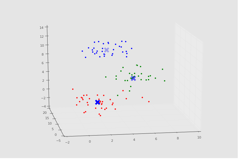
```py
import numpy as np
from sklearn.cluster import MeanShift
from sklearn.datasets.samples_generator import make_blobs
import matplotlib.pyplot as plt
from mpl_toolkits.mplot3d import Axes3D
from matplotlib import style
style.use("ggplot")
centers = [[1,1,1],[5,5,5],[3,10,10]]
X, _ = make_blobs(n_samples = 100, centers = centers, cluster_std = 1.5)
ms = MeanShift()
ms.fit(X)
labels = ms.labels_
cluster_centers = ms.cluster_centers_
print(cluster_centers)
n_clusters_ = len(np.unique(labels))
print("Number of estimated clusters:", n_clusters_)
colors = 10*['r','g','b','c','k','y','m']
fig = plt.figure()
ax = fig.add_subplot(111, projection='3d')
for i in range(len(X)):
ax.scatter(X[i][0], X[i][1], X[i][2], c=colors[labels[i]], marker='o')
ax.scatter(cluster_centers[:,0],cluster_centers[:,1],cluster_centers[:,2],
marker="x",color='k', s=150, linewidths = 5, zorder=10)
plt.show()
```
控制臺輸出:
```
[[ 1.26113946 1.24675516 1.04657994]
[ 4.87468691 4.88157787 5.15456168]
[ 2.77026724 10.3096062 10.40855045]]
Number of estimated clusters: 3
```
繪圖:
## 四十、應用均值漂移的泰坦尼克數據集
歡迎閱讀第四十篇機器學習教程,也是另一篇聚類的教程。我們使用均值漂移,繼續聚類和非監督學習的話題,這次將其用于我們的泰坦尼克數據集。
這里有一些隨機度,所以你的結果可能并不相同,然而你可以重新運行程序來獲取相似結果,如果你沒有得到相似結果的話。
我們打算通過均值漂移聚類來看一看泰坦尼克數據集。我們感興趣的是,是否均值漂移能夠自動將乘客分離為分組。如果能,檢查它創建的分組就很有趣了。第一個明顯的興趣點就是,所發現分組的幸存率,但是,我們也會深入這些分組的屬性,來觀察我們是否能夠理解,均值漂移為什么決定了特定的分組。
首先,我們使用已經看過的代碼:
```py
import numpy as np
from sklearn.cluster import MeanShift, KMeans
from sklearn import preprocessing, cross_validation
import pandas as pd
import matplotlib.pyplot as plt
'''
Pclass Passenger Class (1 = 1st; 2 = 2nd; 3 = 3rd)
survival Survival (0 = No; 1 = Yes)
name Name
sex Sex
age Age
sibsp Number of Siblings/Spouses Aboard
parch Number of Parents/Children Aboard
ticket Ticket Number
fare Passenger Fare (British pound)
cabin Cabin
embarked Port of Embarkation (C = Cherbourg; Q = Queenstown; S = Southampton)
boat Lifeboat
body Body Identification Number
home.dest Home/Destination
'''
# https://pythonprogramming.net/static/downloads/machine-learning-data/titanic.xls
df = pd.read_excel('titanic.xls')
original_df = pd.DataFrame.copy(df)
df.drop(['body','name'], 1, inplace=True)
df.fillna(0,inplace=True)
def handle_non_numerical_data(df):
# handling non-numerical data: must convert.
columns = df.columns.values
for column in columns:
text_digit_vals = {}
def convert_to_int(val):
return text_digit_vals[val]
#print(column,df[column].dtype)
if df[column].dtype != np.int64 and df[column].dtype != np.float64:
column_contents = df[column].values.tolist()
#finding just the uniques
unique_elements = set(column_contents)
# great, found them.
x = 0
for unique in unique_elements:
if unique not in text_digit_vals:
# creating dict that contains new
# id per unique string
text_digit_vals[unique] = x
x+=1
# now we map the new "id" vlaue
# to replace the string.
df[column] = list(map(convert_to_int,df[column]))
return df
df = handle_non_numerical_data(df)
df.drop(['ticket','home.dest'], 1, inplace=True)
X = np.array(df.drop(['survived'], 1).astype(float))
X = preprocessing.scale(X)
y = np.array(df['survived'])
clf = MeanShift()
clf.fit(X)
```
除了兩個例外,一個是`original_df = pd.DataFrame.copy(df)`,在我們將`csv`文件讀取到`df`對象之后。另一個是從`sklearn.cluster `導入`MeanShift`,并且用其作為我們的聚類器。我們生成了副本,以便之后引用原始非數值形式的數據。
既然我們創建了擬合,我們可以從`clf`對象獲取一些屬性。
```py
labels = clf.labels_
cluster_centers = clf.cluster_centers_
```
下面,我們打算向我們的原始數據幀添加新的一項。
```py
original_df['cluster_group']=np.nan
```
現在,我們可以迭代標簽,并向空列添加新的標簽。
```py
for i in range(len(X)):
original_df['cluster_group'].iloc[i] = labels[i]
```
現在我們可以檢查每個分組的幸存率:
```py
n_clusters_ = len(np.unique(labels))
survival_rates = {}
for i in range(n_clusters_):
temp_df = original_df[ (original_df['cluster_group']==float(i)) ]
#print(temp_df.head())
survival_cluster = temp_df[ (temp_df['survived'] == 1) ]
survival_rate = len(survival_cluster) / len(temp_df)
#print(i,survival_rate)
survival_rates[i] = survival_rate
print(survival_rates)
```
如果我們執行它,我們會得到:
```
{0: 0.3796583850931677, 1: 0.9090909090909091, 2: 0.1}
```
同樣,你可能獲得更多分組。我這里獲得了三個,但是我在這個數據集上獲得過六個分組。現在,我們看到分組 0 的幸存率是 38%,分組 1 是 91%,分組 2 是 10%。這就有些奇怪了,因為我們知道船上有三個真實的“乘客分類”。我想知道是不是 0 就是二等艙,1 就是頭等艙, 2 是三等艙。船上的艙是,3 等艙在最底下,頭等艙在最上面,底部首先淹沒,然后頂部是救生船的地方。我可以深入看一看:
```py
print(original_df[ (original_df['cluster_group']==1) ])
```
我們獲取`cluster_group`為 1 的`original_df `。
打印出來:
```py
pclass survived name \
17 1 1 Baxter, Mrs. James (Helene DeLaudeniere Chaput)
49 1 1 Cardeza, Mr. Thomas Drake Martinez
50 1 1 Cardeza, Mrs. James Warburton Martinez (Charlo...
66 1 1 Chaudanson, Miss. Victorine
97 1 1 Douglas, Mrs. Frederick Charles (Mary Helene B...
116 1 1 Fortune, Mrs. Mark (Mary McDougald)
183 1 1 Lesurer, Mr. Gustave J
251 1 1 Ryerson, Miss. Susan Parker "Suzette"
252 1 0 Ryerson, Mr. Arthur Larned
253 1 1 Ryerson, Mrs. Arthur Larned (Emily Maria Borie)
302 1 1 Ward, Miss. Anna
sex age sibsp parch ticket fare cabin embarked \
17 female 50.0 0 1 PC 17558 247.5208 B58 B60 C
49 male 36.0 0 1 PC 17755 512.3292 B51 B53 B55 C
50 female 58.0 0 1 PC 17755 512.3292 B51 B53 B55 C
66 female 36.0 0 0 PC 17608 262.3750 B61 C
97 female 27.0 1 1 PC 17558 247.5208 B58 B60 C
116 female 60.0 1 4 19950 263.0000 C23 C25 C27 S
183 male 35.0 0 0 PC 17755 512.3292 B101 C
251 female 21.0 2 2 PC 17608 262.3750 B57 B59 B63 B66 C
252 male 61.0 1 3 PC 17608 262.3750 B57 B59 B63 B66 C
253 female 48.0 1 3 PC 17608 262.3750 B57 B59 B63 B66 C
302 female 35.0 0 0 PC 17755 512.3292 NaN C
boat body home.dest cluster_group
17 6 NaN Montreal, PQ 1.0
49 3 NaN Austria-Hungary / Germantown, Philadelphia, PA 1.0
50 3 NaN Germantown, Philadelphia, PA 1.0
66 4 NaN NaN 1.0
97 6 NaN Montreal, PQ 1.0
116 10 NaN Winnipeg, MB 1.0
183 3 NaN NaN 1.0
251 4 NaN Haverford, PA / Cooperstown, NY 1.0
252 NaN NaN Haverford, PA / Cooperstown, NY 1.0
253 4 NaN Haverford, PA / Cooperstown, NY 1.0
302 3 NaN NaN 1.0
```
很確定了,整個分組就是頭等艙。也就是說,這里實際上只有 11 個人。讓我們看看分組 0,它看起來有些不同。這一次,我們使用 Pandas 的`.describe()`方法。
```py
print(original_df[ (original_df['cluster_group']==0) ].describe())
```
```
pclass survived age sibsp parch \
count 1288.000000 1288.000000 1027.000000 1288.000000 1288.000000
mean 2.300466 0.379658 29.668614 0.496118 0.332298
std 0.833785 0.485490 14.395610 1.047430 0.686068
min 1.000000 0.000000 0.166700 0.000000 0.000000
25% 2.000000 0.000000 21.000000 0.000000 0.000000
50% 3.000000 0.000000 28.000000 0.000000 0.000000
75% 3.000000 1.000000 38.000000 1.000000 0.000000
max 3.000000 1.000000 80.000000 8.000000 4.000000
fare body cluster_group
count 1287.000000 119.000000 1288.0
mean 30.510172 159.571429 0.0
std 41.511032 97.302914 0.0
min 0.000000 1.000000 0.0
25% 7.895800 71.000000 0.0
50% 14.108300 155.000000 0.0
75% 30.070800 255.500000 0.0
max 263.000000 328.000000 0.0
```
這里有 1287 個人,我們可以看到平均等級是二等艙,但是這里從頭等到三等都有。
讓我們檢查最后一個分組,2,它的預期是全都是三等艙:
```py
print(original_df[ (original_df['cluster_group']==2) ].describe())
```
```
pclass survived age sibsp parch fare \
count 10.0 10.000000 8.000000 10.000000 10.000000 10.000000
mean 3.0 0.100000 39.875000 0.800000 6.000000 42.703750
std 0.0 0.316228 1.552648 0.421637 1.632993 15.590194
min 3.0 0.000000 38.000000 0.000000 5.000000 29.125000
25% 3.0 0.000000 39.000000 1.000000 5.000000 31.303125
50% 3.0 0.000000 39.500000 1.000000 5.000000 35.537500
75% 3.0 0.000000 40.250000 1.000000 6.000000 46.900000
max 3.0 1.000000 43.000000 1.000000 9.000000 69.550000
body cluster_group
count 2.000000 10.0
mean 234.500000 2.0
std 130.814755 0.0
min 142.000000 2.0
25% 188.250000 2.0
50% 234.500000 2.0
75% 280.750000 2.0
max 327.000000 2.0
```
很確定了,我們是對的,這個分組全是三等艙,所以有最壞的幸存率。
足夠有趣,在查看所有分組的時候,分組 2 的票價范圍的確是最低的,從 29 到 69 磅。
在我們查看簇 0 的時候,票價最高為 263 磅。這是最大的組,幸存率為 38%。
當我們回顧簇 1 時,它全是頭等艙,我們看到這里的票價范圍是 247 ~ 512 磅,均值為 350。盡管簇 0 有一些頭等艙的乘客,這個分組是最精英的分組。
出于好奇,分組 0 的頭等艙的生存率,與整體生存率相比如何呢?
```py
>>> cluster_0 = (original_df[ (original_df['cluster_group']==0) ])
>>> cluster_0_fc = (cluster_0[ (cluster_0['pclass']==1) ])
>>> print(cluster_0_fc.describe())
pclass survived age sibsp parch fare \
count 312.0 312.000000 273.000000 312.000000 312.000000 312.000000
mean 1.0 0.608974 39.027167 0.432692 0.326923 78.232519
std 0.0 0.488764 14.589592 0.606997 0.653100 60.300654
min 1.0 0.000000 0.916700 0.000000 0.000000 0.000000
25% 1.0 0.000000 28.000000 0.000000 0.000000 30.500000
50% 1.0 1.000000 39.000000 0.000000 0.000000 58.689600
75% 1.0 1.000000 49.000000 1.000000 0.000000 91.079200
max 1.0 1.000000 80.000000 3.000000 4.000000 263.000000
body cluster_group
count 35.000000 312.0
mean 162.828571 0.0
std 82.652172 0.0
min 16.000000 0.0
25% 109.500000 0.0
50% 166.000000 0.0
75% 233.000000 0.0
max 307.000000 0.0
>>>
```
很確定了,它們的幸存率更高,約為 61%,但是仍然低于精英分組(根據票價和幸存率)的 91%。花費一些時間來深入挖掘,看看你是否能發現一些東西。然后我們要到下一章,自己編寫均值漂移算法。
## 四十一、從零編寫均值漂移
> 原文:[Mean Shift algorithm from scratch in Python
](https://pythonprogramming.net/mean-shift-from-scratch-python-machine-learning-tutorial/)
歡迎閱讀第四十一篇教程,這是另一篇聚類教程。
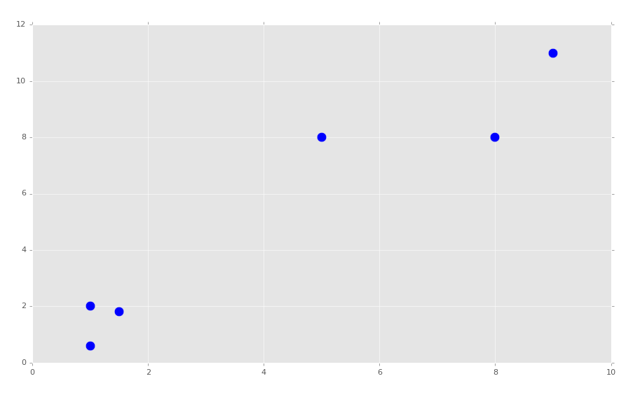
這篇教程中,我們從零開始構建我們自己的均值漂移算法。首先,我們會以一些 37 章中的代碼開始,它就是我們開始構建 KMeans 算法的地方。我會向原始原始數據添加更多簇或者分組。你可以添加新的數據,或者保留原樣。
```py
import matplotlib.pyplot as plt
from matplotlib import style
style.use('ggplot')
import numpy as np
X = np.array([[1, 2],
[1.5, 1.8],
[5, 8 ],
[8, 8],
[1, 0.6],
[9,11],
[8,2],
[10,2],
[9,3],])
plt.scatter(X[:,0], X[:,1], s=150)
plt.show()
colors = 10*["g","r","c","b","k"]
```
運行之后,代碼會生成:
就像 KMeans 那部分,這會創建明顯的分組。對于 KMeans,我們告訴機器我們想要 K(2)個簇。對于均值漂移,我們希望機器自己識別出來,并且對于我們來說,我們希望有三個分組。
我們開始我們的`MeanShift`類:
```py
class Mean_Shift:
def __init__(self, radius=4):
self.radius = radius
```
我們會以半徑 4 開始,因為我們可以估計出,半徑 4 是有意義的。這就是我們在初始化方法中需要的所有東西。我們來看看`fit`方法:
```py
def fit(self, data):
centroids = {}
for i in range(len(data)):
centroids[i] = data[i]
```
這里,我們開始創建起始形心。均值漂移的方法是:
1. 讓所有數據點都是形心。
2. 計算形心半徑內的所有數據集,將均值設置為新的形心。
3. 重復步驟 2 直至收斂。
目前為止,我們完成了步驟 1,現在需要重復步驟 2 直到收斂。
```py
while True:
new_centroids = []
for i in centroids:
in_bandwidth = []
centroid = centroids[i]
for featureset in data:
if np.linalg.norm(featureset-centroid) < self.radius:
in_bandwidth.append(featureset)
new_centroid = np.average(in_bandwidth,axis=0)
new_centroids.append(tuple(new_centroid))
uniques = sorted(list(set(new_centroids)))
```
這里,我們開始迭代每個形心,并且找到范圍內的所有特征集。這里,我們計算了均值,并將均值設置為新的形心。最后,我們創建`unique`變量,它跟蹤了所有已知形心的排序后的列表。我們這里使用`set`,因為它們可能重復,重復的形心也就是同一個形心。
我們來完成`fit`方法:
```py
prev_centroids = dict(centroids)
centroids = {}
for i in range(len(uniques)):
centroids[i] = np.array(uniques[i])
optimized = True
for i in centroids:
if not np.array_equal(centroids[i], prev_centroids[i]):
optimized = False
if not optimized:
break
if optimized:
break
self.centroids = centroids
```
這里我們注意到之前的形心,之后,我們重置“當前”或者“新的”形心,通過將其去重。最后,我們比較了之前的形心和新的形心,并度量了移動。如果任何形心發生了移動,就不是完全收斂和最優化,我們就需要繼續執行另一個循環。如果它是最優化的,我們就終端,之后將`centroids`屬性設置為我們生成的最后一個形心。
我們現在可以將這個第一個部分,以及類包裝起來,添加下面這些東西:
```py
clf = Mean_Shift()
clf.fit(X)
centroids = clf.centroids
plt.scatter(X[:,0], X[:,1], s=150)
for c in centroids:
plt.scatter(centroids[c][0], centroids[c][1], color='k', marker='*', s=150)
plt.show()
```
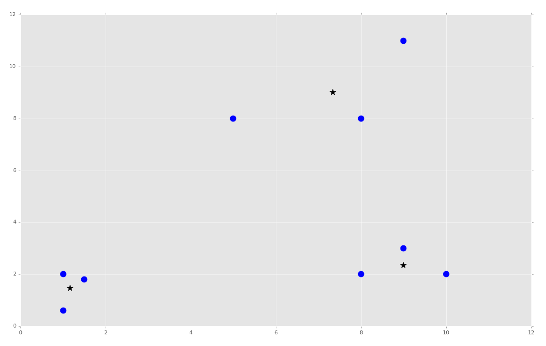
目前為止的完整代碼:
```py
import matplotlib.pyplot as plt
from matplotlib import style
style.use('ggplot')
import numpy as np
X = np.array([[1, 2],
[1.5, 1.8],
[5, 8 ],
[8, 8],
[1, 0.6],
[9,11],
[8,2],
[10,2],
[9,3],])
##plt.scatter(X[:,0], X[:,1], s=150)
##plt.show()
colors = 10*["g","r","c","b","k"]
class Mean_Shift:
def __init__(self, radius=4):
self.radius = radius
def fit(self, data):
centroids = {}
for i in range(len(data)):
centroids[i] = data[i]
while True:
new_centroids = []
for i in centroids:
in_bandwidth = []
centroid = centroids[i]
for featureset in data:
if np.linalg.norm(featureset-centroid) < self.radius:
in_bandwidth.append(featureset)
new_centroid = np.average(in_bandwidth,axis=0)
new_centroids.append(tuple(new_centroid))
uniques = sorted(list(set(new_centroids)))
prev_centroids = dict(centroids)
centroids = {}
for i in range(len(uniques)):
centroids[i] = np.array(uniques[i])
optimized = True
for i in centroids:
if not np.array_equal(centroids[i], prev_centroids[i]):
optimized = False
if not optimized:
break
if optimized:
break
self.centroids = centroids
clf = Mean_Shift()
clf.fit(X)
centroids = clf.centroids
plt.scatter(X[:,0], X[:,1], s=150)
for c in centroids:
plt.scatter(centroids[c][0], centroids[c][1], color='k', marker='*', s=150)
plt.show()
```
到這里,我們獲取了所需的形心,并且我們覺得十分聰明。從此,所有我們所需的就是計算歐氏距離,并且我們擁有了形心和分類。預測就變得簡單了。現在只有一個問題:半徑。
我們基本上硬編碼了半徑。我看了數據集之后才決定 4 是個好的數值。這一點也不動態,并且它不像是非監督機器學習。假設如果我們有 50 個維度呢?就不會很簡單了。機器能夠觀察數據集并得出合理的值嗎?我們會在下一個教程中涉及它。
## 四十二、均值漂移的動態權重帶寬
歡迎閱讀第四十二篇教程,另一篇聚類的教程。我們打算繼續處理我們自己的均值漂移算法。
目前為止的代碼:
```py
import matplotlib.pyplot as plt
from matplotlib import style
style.use('ggplot')
import numpy as np
X = np.array([[1, 2],
[1.5, 1.8],
[5, 8 ],
[8, 8],
[1, 0.6],
[9,11],
[8,2],
[10,2],
[9,3],])
##plt.scatter(X[:,0], X[:,1], s=150)
##plt.show()
colors = 10*["g","r","c","b","k"]
class Mean_Shift:
def __init__(self, radius=4):
self.radius = radius
def fit(self, data):
centroids = {}
for i in range(len(data)):
centroids[i] = data[i]
while True:
new_centroids = []
for i in centroids:
in_bandwidth = []
centroid = centroids[i]
for featureset in data:
if np.linalg.norm(featureset-centroid) < self.radius:
in_bandwidth.append(featureset)
new_centroid = np.average(in_bandwidth,axis=0)
new_centroids.append(tuple(new_centroid))
uniques = sorted(list(set(new_centroids)))
prev_centroids = dict(centroids)
centroids = {}
for i in range(len(uniques)):
centroids[i] = np.array(uniques[i])
optimized = True
for i in centroids:
if not np.array_equal(centroids[i], prev_centroids[i]):
optimized = False
if not optimized:
break
if optimized:
break
self.centroids = centroids
clf = Mean_Shift()
clf.fit(X)
centroids = clf.centroids
plt.scatter(X[:,0], X[:,1], s=150)
for c in centroids:
plt.scatter(centroids[c][0], centroids[c][1], color='k', marker='*', s=150)
plt.show()
```
這個代碼能夠工作,但是我們決定硬編碼的半徑不好。我們希望做一些更好的事情。首先,我們會修改我們的`__init__`方法:
```py
def __init__(self, radius=None, radius_norm_step = 100):
self.radius = radius
self.radius_norm_step = radius_norm_step
```
所以這里的計劃時創建大量的半徑,但是逐步處理這個半徑,就像帶寬一樣,或者一些不同長度的半徑,我們將其稱為步驟。如果特征集靠近半徑,它就比遠離的點有更大的“權重”。唯一的問題就是,這些步驟應該是什么。現在,開始實現我們的方法:
```py
def fit(self, data):
if self.radius == None:
all_data_centroid = np.average(data, axis=0)
all_data_norm = np.linalg.norm(all_data_centroid)
self.radius = all_data_norm / self.radius_norm_step
centroids = {}
for i in range(len(data)):
centroids[i] = data[i]
```
這里,如果用戶沒有硬編碼半徑,我們就打算尋找所有數據的“中心”。之后,我們會計算數據的模,之后假設每個`self.radius`中的半徑都是整個數據長度,再除以我們希望的步驟數量。這里,形心的定義和上面的代碼相同。現在我們開始`while`循環的優化:
```py
weights = [i for i in range(self.radius_norm_step)][::-1]
while True:
new_centroids = []
for i in centroids:
in_bandwidth = []
centroid = centroids[i]
for featureset in data:
#if np.linalg.norm(featureset-centroid) < self.radius:
# in_bandwidth.append(featureset)
distance = np.linalg.norm(featureset-centroid)
if distance == 0:
distance = 0.00000000001
weight_index = int(distance/self.radius)
if weight_index > self.radius_norm_step-1:
weight_index = self.radius_norm_step-1
to_add = (weights[weight_index]**2)*[featureset]
in_bandwidth +=to_add
new_centroid = np.average(in_bandwidth,axis=0)
new_centroids.append(tuple(new_centroid))
uniques = sorted(list(set(new_centroids)))
```
要注意權重的定義,之后是數據中特征集的改變。
