# PythonProgramming.net 自然語言處理教程
> 原文:[Natural Language Process](https://pythonprogramming.net/tokenizing-words-sentences-nltk-tutorial/)
> 譯者:[飛龍](https://github.com/)
> 協議:[CC BY-NC-SA 4.0](http://creativecommons.org/licenses/by-nc-sa/4.0/)
# 一、使用 NLTK 分析單詞和句子
歡迎閱讀自然語言處理系列教程,使用 Python 的自然語言工具包 NLTK 模塊。
NLTK 模塊是一個巨大的工具包,目的是在整個自然語言處理(NLP)方法上幫助你。 NLTK 將為你提供一切,從將段落拆分為句子,拆分詞語,識別這些詞語的詞性,高亮主題,甚至幫助你的機器了解文本關于什么。在這個系列中,我們將要解決意見挖掘或情感分析的領域。
在我們學習如何使用 NLTK 進行情感分析的過程中,我們將學習以下內容:
+ 分詞 - 將文本正文分割為句子和單詞。
+ 詞性標注
+ 機器學習與樸素貝葉斯分類器
+ 如何一起使用 Scikit Learn(sklearn)與 NLTK
+ 用數據集訓練分類器
+ 用 Twitter 進行實時的流式情感分析。
+ ...以及更多。
為了開始,你需要 NLTK 模塊,以及 Python。
如果你還沒有 Python,請轉到`python.org`并下載最新版本的 Python(如果你在 Windows上)。如果你在 Mac 或 Linux 上,你應該可以運行`apt-get install python3`。
接下來,你需要 NLTK 3。安裝 NLTK 模塊的最簡單方法是使用`pip`。
對于所有的用戶來說,這通過打開`cmd.exe`,bash,或者你使用的任何 shell,并鍵入以下命令來完成:
```
pip install nltk
```
接下來,我們需要為 NLTK 安裝一些組件。通過你的任何常用方式打開 python,然后鍵入:
```py
import nltk
nltk.download()
```
除非你正在操作無頭版本,否則一個 GUI 會彈出來,可能只有紅色而不是綠色:
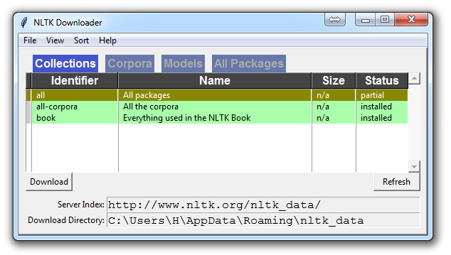
為所有軟件包選擇下載“全部”,然后單擊“下載”。 這會給你所有分詞器,分塊器,其他算法和所有的語料庫。 如果空間是個問題,你可以選擇手動選擇性下載所有內容。 NLTK 模塊將占用大約 7MB,整個`nltk_data`目錄將占用大約 1.8GB,其中包括你的分塊器,解析器和語料庫。
如果你正在使用 VPS 運行無頭版本,你可以通過運行 Python ,并執行以下操作來安裝所有內容:
```py
import nltk
nltk.download()
d (for download)
all (for download everything)
```
這將為你下載一切東西。
現在你已經擁有了所有你需要的東西,讓我們敲一些簡單的詞匯:
+ 語料庫(Corpus) - 文本的正文,單數。Corpora 是它的復數。示例:`A collection of medical journals`。
+ 詞庫(Lexicon) - 詞匯及其含義。例如:英文字典。但是,考慮到各個領域會有不同的詞庫。例如:對于金融投資者來說,`Bull`(牛市)這個詞的第一個含義是對市場充滿信心的人,與“普通英語詞匯”相比,這個詞的第一個含義是動物。因此,金融投資者,醫生,兒童,機械師等都有一個特殊的詞庫。
+ 標記(Token) - 每個“實體”都是根據規則分割的一部分。例如,當一個句子被“拆分”成單詞時,每個單詞都是一個標記。如果你將段落拆分為句子,則每個句子也可以是一個標記。
這些是在進入自然語言處理(NLP)領域時,最常聽到的詞語,但是我們將及時涵蓋更多的詞匯。以此,我們來展示一個例子,說明如何用 NLTK 模塊將某些東西拆分為標記。
```py
from nltk.tokenize import sent_tokenize, word_tokenize
EXAMPLE_TEXT = "Hello Mr. Smith, how are you doing today? The weather is great, and Python is awesome. The sky is pinkish-blue. You shouldn't eat cardboard."
print(sent_tokenize(EXAMPLE_TEXT))
```
起初,你可能會認為按照詞或句子來分詞,是一件相當微不足道的事情。 對于很多句子來說,它可能是。 第一步可能是執行一個簡單的`.split('. ')`,或按照句號,然后是空格分割。 之后也許你會引入一些正則表達式,來按照句號,空格,然后是大寫字母分割。 問題是像`Mr. Smith`這樣的事情,還有很多其他的事情會給你帶來麻煩。 按照詞分割也是一個挑戰,特別是在考慮縮寫的時候,例如`we`和`we're`。 NLTK 用這個看起來簡單但非常復雜的操作為你節省大量的時間。
上面的代碼會輸出句子,分成一個句子列表,你可以用`for`循環來遍歷。
```py
['Hello Mr. Smith, how are you doing today?', 'The weather is great, and Python is awesome.', 'The sky is pinkish-blue.', "You shouldn't eat cardboard."]
```
所以這里,我們創建了標記,它們都是句子。讓我們這次按照詞來分詞。
```py
print(word_tokenize(EXAMPLE_TEXT))
['Hello', 'Mr.', 'Smith', ',', 'how', 'are', 'you', 'doing', 'today', '?', 'The', 'weather', 'is', 'great', ',', 'and', 'Python', 'is', 'awesome', '.', 'The', 'sky', 'is', 'pinkish-blue', '.', 'You', 'should', "n't", 'eat', 'cardboard', '.']
```
這里有幾件事要注意。 首先,注意標點符號被視為一個單獨的標記。 另外,注意單詞`shouldn't`分隔為`should`和`n't`。 最后要注意的是,`pinkish-blue`確實被當作“一個詞”來對待,本來就是這樣。很酷!
現在,看著這些分詞后的單詞,我們必須開始思考我們的下一步可能是什么。 我們開始思考如何通過觀察這些詞匯來獲得含義。 我們可以想清楚,如何把價值放在許多單詞上,但我們也看到一些基本上毫無價值的單詞。 這是一種“停止詞”的形式,我們也可以處理。 這就是我們將在下一個教程中討論的內容。
## 二、NLTK 與停止詞
自然語言處理的思想,是進行某種形式的分析或處理,機器至少可以在某種程度上理解文本的含義,表述或暗示。
這顯然是一個巨大的挑戰,但是有一些任何人都能遵循的步驟。然而,主要思想是電腦根本不會直接理解單詞。令人震驚的是,人類也不會。在人類中,記憶被分解成大腦中的電信號,以發射模式的神經組的形式。對于大腦還有很多未知的事情,但是我們越是把人腦分解成基本的元素,我們就會發現基本的元素。那么,事實證明,計算機以非常相似的方式存儲信息!如果我們要模仿人類如何閱讀和理解文本,我們需要一種盡可能接近的方法。一般來說,計算機使用數字來表示一切事物,但是我們經常直接在編程中看到使用二進制信號(`True`或`False`,可以直接轉換為 1 或 0,直接來源于電信號存在`(True, 1)`或不存在`(False, 0)`)。為此,我們需要一種方法,將單詞轉換為數值或信號模式。將數據轉換成計算機可以理解的東西,這個過程稱為“預處理”。預處理的主要形式之一就是過濾掉無用的數據。在自然語言處理中,無用詞(數據)被稱為停止詞。
我們可以立即認識到,有些詞語比其他詞語更有意義。我們也可以看到,有些單詞是無用的,是填充詞。例如,我們在英語中使用它們來填充句子,這樣就沒有那么奇怪的聲音了。一個最常見的,非官方的,無用詞的例子是單詞`umm`。人們經常用`umm`來填充,比別的詞多一些。這個詞毫無意義,除非我們正在尋找一個可能缺乏自信,困惑,或者說沒有太多話的人。我們都這樣做,有...呃...很多時候,你可以在視頻中聽到我說`umm`或`uhh`。對于大多數分析而言,這些詞是無用的。
我們不希望這些詞占用我們數據庫的空間,或占用寶貴的處理時間。因此,我們稱這些詞為“無用詞”,因為它們是無用的,我們希望對它們不做處理。 “停止詞”這個詞的另一個版本可以更書面一些:我們停在上面的單詞。
例如,如果你發現通常用于諷刺的詞語,可能希望立即停止。諷刺的單詞或短語將因詞庫和語料庫而異。就目前而言,我們將把停止詞當作不含任何含義的詞,我們要把它們刪除。
你可以輕松地實現它,通過存儲你認為是停止詞的單詞列表。 NLTK 用一堆他們認為是停止詞的單詞,來讓你起步,你可以通過 NLTK 語料庫來訪問它:
```py
from nltk.corpus import stopwords
```
這里是這個列表:
```py
>>> set(stopwords.words('english'))
{'ourselves', 'hers', 'between', 'yourself', 'but', 'again', 'there', 'about', 'once', 'during', 'out', 'very', 'having', 'with', 'they', 'own', 'an', 'be', 'some', 'for', 'do', 'its', 'yours', 'such', 'into', 'of', 'most', 'itself', 'other', 'off', 'is', 's', 'am', 'or', 'who', 'as', 'from', 'him', 'each', 'the', 'themselves', 'until', 'below', 'are', 'we', 'these', 'your', 'his', 'through', 'don', 'nor', 'me', 'were', 'her', 'more', 'himself', 'this', 'down', 'should', 'our', 'their', 'while', 'above', 'both', 'up', 'to', 'ours', 'had', 'she', 'all', 'no', 'when', 'at', 'any', 'before', 'them', 'same', 'and', 'been', 'have', 'in', 'will', 'on', 'does', 'yourselves', 'then', 'that', 'because', 'what', 'over', 'why', 'so', 'can', 'did', 'not', 'now', 'under', 'he', 'you', 'herself', 'has', 'just', 'where', 'too', 'only', 'myself', 'which', 'those', 'i', 'after', 'few', 'whom', 't', 'being', 'if', 'theirs', 'my', 'against', 'a', 'by', 'doing', 'it', 'how', 'further', 'was', 'here', 'than'}
```
以下是結合使用`stop_words`集合,從文本中刪除停止詞的方法:
```py
from nltk.corpus import stopwords
from nltk.tokenize import word_tokenize
example_sent = "This is a sample sentence, showing off the stop words filtration."
stop_words = set(stopwords.words('english'))
word_tokens = word_tokenize(example_sent)
filtered_sentence = [w for w in word_tokens if not w in stop_words]
filtered_sentence = []
for w in word_tokens:
if w not in stop_words:
filtered_sentence.append(w)
print(word_tokens)
print(filtered_sentence)
```
我們的輸出是:
```py
['This', 'is', 'a', 'sample', 'sentence', ',', 'showing', 'off', 'the', 'stop', 'words', 'filtration', '.']
['This', 'sample', 'sentence', ',', 'showing', 'stop', 'words', 'filtration', '.']
```
我們的數據庫感謝了我們。數據預處理的另一種形式是“詞干提取(Stemming)”,這就是我們接下來要討論的內容。
## 三、NLTK 詞干提取
詞干的概念是一種規范化方法。 除涉及時態之外,許多詞語的變體都具有相同的含義。
我們提取詞干的原因是為了縮短查找的時間,使句子正常化。
考慮:
```
I was taking a ride in the car.
I was riding in the car.
```
這兩句話意味著同樣的事情。 `in the car`(在車上)是一樣的。 `I`(我)是一樣的。 在這兩種情況下,`ing`都明確表示過去式,所以在試圖弄清這個過去式活動的含義的情況下,是否真的有必要區分`riding`和`taking a ride`?
不,并沒有。
這只是一個小例子,但想象英語中的每個單詞,可以放在單詞上的每個可能的時態和詞綴。 每個版本有單獨的字典條目,將非常冗余和低效,特別是因為一旦我們轉換為數字,“價值”將是相同的。
最流行的瓷感提取算法之一是 Porter,1979 年就存在了。
首先,我們要抓取并定義我們的詞干:
```py
from nltk.stem import PorterStemmer
from nltk.tokenize import sent_tokenize, word_tokenize
ps = PorterStemmer()
```
現在讓我們選擇一些帶有相似詞干的單詞,例如:
```py
example_words = ["python","pythoner","pythoning","pythoned","pythonly"]
```
下面,我們可以這樣做來輕易提取詞干:
```py
for w in example_words:
print(ps.stem(w))
```
我們的輸出:
```py
python
python
python
python
pythonli
```
現在讓我們嘗試對一個典型的句子,而不是一些單詞提取詞干:
```py
new_text = "It is important to by very pythonly while you are pythoning with python. All pythoners have pythoned poorly at least once."
words = word_tokenize(new_text)
for w in words:
print(ps.stem(w))
```
現在我們的結果為:
```
It
is
import
to
by
veri
pythonli
while
you
are
python
with
python
.
All
python
have
python
poorli
at
least
onc
.
```
接下來,我們將討論 NLTK 模塊中一些更高級的內容,詞性標注,其中我們可以使用 NLTK 模塊來識別句子中每個單詞的詞性。
## 四、NLTK 詞性標注
NLTK模塊的一個更強大的方面是,它可以為你做詞性標注。 意思是把一個句子中的單詞標注為名詞,形容詞,動詞等。 更令人印象深刻的是,它也可以按照時態來標記,以及其他。 這是一列標簽,它們的含義和一些例子:
```py
POS tag list:
CC coordinating conjunction
CD cardinal digit
DT determiner
EX existential there (like: "there is" ... think of it like "there exists")
FW foreign word
IN preposition/subordinating conjunction
JJ adjective 'big'
JJR adjective, comparative 'bigger'
JJS adjective, superlative 'biggest'
LS list marker 1)
MD modal could, will
NN noun, singular 'desk'
NNS noun plural 'desks'
NNP proper noun, singular 'Harrison'
NNPS proper noun, plural 'Americans'
PDT predeterminer 'all the kids'
POS possessive ending parent's
PRP personal pronoun I, he, she
PRP$ possessive pronoun my, his, hers
RB adverb very, silently,
RBR adverb, comparative better
RBS adverb, superlative best
RP particle give up
TO to go 'to' the store.
UH interjection errrrrrrrm
VB verb, base form take
VBD verb, past tense took
VBG verb, gerund/present participle taking
VBN verb, past participle taken
VBP verb, sing. present, non-3d take
VBZ verb, 3rd person sing. present takes
WDT wh-determiner which
WP wh-pronoun who, what
WP$ possessive wh-pronoun whose
WRB wh-abverb where, when
```
我們如何使用這個? 當我們處理它的時候,我們要講解一個新的句子標記器,叫做`PunktSentenceTokenizer`。 這個標記器能夠無監督地進行機器學習,所以你可以在你使用的任何文本上進行實際的訓練。 首先,讓我們獲取一些我們打算使用的導入:
```py
import nltk
from nltk.corpus import state_union
from nltk.tokenize import PunktSentenceTokenizer
```
現在讓我們創建訓練和測試數據:
```py
train_text = state_union.raw("2005-GWBush.txt")
sample_text = state_union.raw("2006-GWBush.txt")
```
一個是 2005 年以來的國情咨文演說,另一個是 2006 年以來的喬治·W·布什總統的演講。
接下來,我們可以訓練 Punkt 標記器,如下所示:
```py
custom_sent_tokenizer = PunktSentenceTokenizer(train_text)
```
之后我們可以實際分詞,使用:
```py
tokenized = custom_sent_tokenizer.tokenize(sample_text)
```
現在我們可以通過創建一個函數,來完成這個詞性標注腳本,該函數將遍歷并標記每個句子的詞性,如下所示:
```py
def process_content():
try:
for i in tokenized[:5]:
words = nltk.word_tokenize(i)
tagged = nltk.pos_tag(words)
print(tagged)
except Exception as e:
print(str(e))
process_content()
```
輸出應該是元組列表,元組中的第一個元素是單詞,第二個元素是詞性標簽。 它應該看起來像:
```py
[('PRESIDENT', 'NNP'), ('GEORGE', 'NNP'), ('W.', 'NNP'), ('BUSH', 'NNP'), ("'S", 'POS'), ('ADDRESS', 'NNP'), ('BEFORE', 'NNP'), ('A', 'NNP'), ('JOINT', 'NNP'), ('SESSION', 'NNP'), ('OF', 'NNP'), ('THE', 'NNP'), ('CONGRESS', 'NNP'), ('ON', 'NNP'), ('THE', 'NNP'), ('STATE', 'NNP'), ('OF', 'NNP'), ('THE', 'NNP'), ('UNION', 'NNP'), ('January', 'NNP'), ('31', 'CD'), (',', ','), ('2006', 'CD'), ('THE', 'DT'), ('PRESIDENT', 'NNP'), (':', ':'), ('Thank', 'NNP'), ('you', 'PRP'), ('all', 'DT'), ('.', '.')] [('Mr.', 'NNP'), ('Speaker', 'NNP'), (',', ','), ('Vice', 'NNP'), ('President', 'NNP'), ('Cheney', 'NNP'), (',', ','), ('members', 'NNS'), ('of', 'IN'), ('Congress', 'NNP'), (',', ','), ('members', 'NNS'), ('of', 'IN'), ('the', 'DT'), ('Supreme', 'NNP'), ('Court', 'NNP'), ('and', 'CC'), ('diplomatic', 'JJ'), ('corps', 'NNS'), (',', ','), ('distinguished', 'VBD'), ('guests', 'NNS'), (',', ','), ('and', 'CC'), ('fellow', 'JJ'), ('citizens', 'NNS'), (':', ':'), ('Today', 'NN'), ('our', 'PRP$'), ('nation', 'NN'), ('lost', 'VBD'), ('a', 'DT'), ('beloved', 'VBN'), (',', ','), ('graceful', 'JJ'), (',', ','), ('courageous', 'JJ'), ('woman', 'NN'), ('who', 'WP'), ('called', 'VBN'), ('America', 'NNP'), ('to', 'TO'), ('its', 'PRP$'), ('founding', 'NN'), ('ideals', 'NNS'), ('and', 'CC'), ('carried', 'VBD'), ('on', 'IN'), ('a', 'DT'), ('noble', 'JJ'), ('dream', 'NN'), ('.', '.')] [('Tonight', 'NNP'), ('we', 'PRP'), ('are', 'VBP'), ('comforted', 'VBN'), ('by', 'IN'), ('the', 'DT'), ('hope', 'NN'), ('of', 'IN'), ('a', 'DT'), ('glad', 'NN'), ('reunion', 'NN'), ('with', 'IN'), ('the', 'DT'), ('husband', 'NN'), ('who', 'WP'), ('was', 'VBD'), ('taken', 'VBN'), ('so', 'RB'), ('long', 'RB'), ('ago', 'RB'), (',', ','), ('and', 'CC'), ('we', 'PRP'), ('are', 'VBP'), ('grateful', 'JJ'), ('for', 'IN'), ('the', 'DT'), ('good', 'NN'), ('life', 'NN'), ('of', 'IN'), ('Coretta', 'NNP'), ('Scott', 'NNP'), ('King', 'NNP'), ('.', '.')] [('(', 'NN'), ('Applause', 'NNP'), ('.', '.'), (')', ':')] [('President', 'NNP'), ('George', 'NNP'), ('W.', 'NNP'), ('Bush', 'NNP'), ('reacts', 'VBZ'), ('to', 'TO'), ('applause', 'VB'), ('during', 'IN'), ('his', 'PRP$'), ('State', 'NNP'), ('of', 'IN'), ('the', 'DT'), ('Union', 'NNP'), ('Address', 'NNP'), ('at', 'IN'), ('the', 'DT'), ('Capitol', 'NNP'), (',', ','), ('Tuesday', 'NNP'), (',', ','), ('Jan', 'NNP'), ('.', '.')]
```
到了這里,我們可以開始獲得含義,但是還有一些工作要做。 我們將要討論的下一個話題是分塊(chunking),其中我們跟句單詞的詞性,將單詞分到,有意義的分組中。
## 五、NLTK 分塊
現在我們知道了詞性,我們可以注意所謂的分塊,把詞匯分成有意義的塊。 分塊的主要目標之一是將所謂的“名詞短語”分組。 這些是包含一個名詞的一個或多個單詞的短語,可能是一些描述性詞語,也可能是一個動詞,也可能是一個副詞。 這個想法是把名詞和與它們有關的詞組合在一起。
為了分塊,我們將詞性標簽與正則表達式結合起來。 主要從正則表達式中,我們要利用這些東西:
```
+ = match 1 or more
? = match 0 or 1 repetitions.
* = match 0 or MORE repetitions
. = Any character except a new line
```
如果你需要正則表達式的幫助,請參閱上面鏈接的教程。 最后需要注意的是,詞性標簽中用`<`和`>`表示,我們也可以在標簽本身中放置正則表達式,來表達“全部名詞”(`<N.*>`)。
```py
import nltk
from nltk.corpus import state_union
from nltk.tokenize import PunktSentenceTokenizer
train_text = state_union.raw("2005-GWBush.txt")
sample_text = state_union.raw("2006-GWBush.txt")
custom_sent_tokenizer = PunktSentenceTokenizer(train_text)
tokenized = custom_sent_tokenizer.tokenize(sample_text)
def process_content():
try:
for i in tokenized:
words = nltk.word_tokenize(i)
tagged = nltk.pos_tag(words)
chunkGram = r"""Chunk: {<RB.?>*<VB.?>*<NNP>+<NN>?}"""
chunkParser = nltk.RegexpParser(chunkGram)
chunked = chunkParser.parse(tagged)
chunked.draw()
except Exception as e:
print(str(e))
process_content()
```
結果是這樣的:
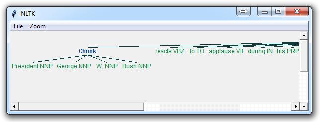
這里的主要一行是:
```py
chunkGram = r"""Chunk: {<RB.?>*<VB.?>*<NNP>+<NN>?}"""
```
把這一行拆分開:
`<RB.?>*`:零個或多個任何時態的副詞,后面是:
`<VB.?>*`:零個或多個任何時態的動詞,后面是:
`<NNP>+`:一個或多個合理的名詞,后面是:
`<NN>?`:零個或一個名詞單數。
嘗試玩轉組合來對各種實例進行分組,直到你覺得熟悉了。
視頻中沒有涉及,但是也有個合理的任務是實際訪問具體的塊。 這是很少被提及的,但根據你在做的事情,這可能是一個重要的步驟。 假設你把塊打印出來,你會看到如下輸出:
```
(S
(Chunk PRESIDENT/NNP GEORGE/NNP W./NNP BUSH/NNP)
'S/POS
(Chunk
ADDRESS/NNP
BEFORE/NNP
A/NNP
JOINT/NNP
SESSION/NNP
OF/NNP
THE/NNP
CONGRESS/NNP
ON/NNP
THE/NNP
STATE/NNP
OF/NNP
THE/NNP
UNION/NNP
January/NNP)
31/CD
,/,
2006/CD
THE/DT
(Chunk PRESIDENT/NNP)
:/:
(Chunk Thank/NNP)
you/PRP
all/DT
./.)
```
很酷,這可以幫助我們可視化,但如果我們想通過我們的程序訪問這些數據呢? 那么,這里發生的是我們的“分塊”變量是一個 NLTK 樹。 每個“塊”和“非塊”是樹的“子樹”。 我們可以通過像`chunked.subtrees`的東西來引用它們。 然后我們可以像這樣遍歷這些子樹:
```py
for subtree in chunked.subtrees():
print(subtree)
```
接下來,我們可能只關心獲得這些塊,忽略其余部分。 我們可以在`chunked.subtrees()`調用中使用`filter`參數。
```py
for subtree in chunked.subtrees(filter=lambda t: t.label() == 'Chunk'):
print(subtree)
```
現在,我們執行過濾,來顯示標簽為“塊”的子樹。 請記住,這不是 NLTK 塊屬性中的“塊”...這是字面上的“塊”,因為這是我們給它的標簽:`chunkGram = r"""Chunk: {<RB.?>*<VB.?>*<NNP>+<NN>?}"""`。
如果我們寫了一些東西,類似`chunkGram = r"""Pythons: {<RB.?>*<VB.?>*<NNP>+<NN>?}"""`,那么我們可以通過`"Pythons."`標簽來過濾。 結果應該是這樣的:
```
-
(Chunk PRESIDENT/NNP GEORGE/NNP W./NNP BUSH/NNP)
(Chunk
ADDRESS/NNP
BEFORE/NNP
A/NNP
JOINT/NNP
SESSION/NNP
OF/NNP
THE/NNP
CONGRESS/NNP
ON/NNP
THE/NNP
STATE/NNP
OF/NNP
THE/NNP
UNION/NNP
January/NNP)
(Chunk PRESIDENT/NNP)
(Chunk Thank/NNP)
```
完整的代碼是:
```py
import nltk
from nltk.corpus import state_union
from nltk.tokenize import PunktSentenceTokenizer
train_text = state_union.raw("2005-GWBush.txt")
sample_text = state_union.raw("2006-GWBush.txt")
custom_sent_tokenizer = PunktSentenceTokenizer(train_text)
tokenized = custom_sent_tokenizer.tokenize(sample_text)
def process_content():
try:
for i in tokenized:
words = nltk.word_tokenize(i)
tagged = nltk.pos_tag(words)
chunkGram = r"""Chunk: {<RB.?>*<VB.?>*<NNP>+<NN>?}"""
chunkParser = nltk.RegexpParser(chunkGram)
chunked = chunkParser.parse(tagged)
print(chunked)
for subtree in chunked.subtrees(filter=lambda t: t.label() == 'Chunk'):
print(subtree)
chunked.draw()
except Exception as e:
print(str(e))
process_content()
```
## 六、 NLTK 添加縫隙(Chinking)
你可能會發現,經過大量的分塊之后,你的塊中還有一些你不想要的單詞,但是你不知道如何通過分塊來擺脫它們。 你可能會發現添加縫隙是你的解決方案。
添加縫隙與分塊很像,它基本上是一種從塊中刪除塊的方法。 你從塊中刪除的塊就是你的縫隙。
代碼非常相似,你只需要用`}{`來代碼縫隙,在塊后面,而不是塊的`{}`。
```py
import nltk
from nltk.corpus import state_union
from nltk.tokenize import PunktSentenceTokenizer
train_text = state_union.raw("2005-GWBush.txt")
sample_text = state_union.raw("2006-GWBush.txt")
custom_sent_tokenizer = PunktSentenceTokenizer(train_text)
tokenized = custom_sent_tokenizer.tokenize(sample_text)
def process_content():
try:
for i in tokenized[5:]:
words = nltk.word_tokenize(i)
tagged = nltk.pos_tag(words)
chunkGram = r"""Chunk: {<.*>+}
}<VB.?|IN|DT|TO>+{"""
chunkParser = nltk.RegexpParser(chunkGram)
chunked = chunkParser.parse(tagged)
chunked.draw()
except Exception as e:
print(str(e))
process_content()
```
使用它,你得到了一些東西:
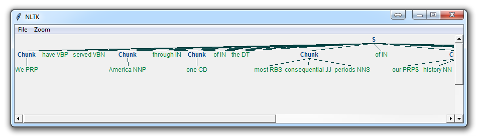
現在,主要的區別是:
```
}<VB.?|IN|DT|TO>+{
```
這意味著我們要從縫隙中刪除一個或多個動詞,介詞,限定詞或`to`這個詞。
現在我們已經學會了,如何執行一些自定義的分塊和添加縫隙,我們來討論一下 NLTK 自帶的分塊形式,這就是命名實體識別。
## 七、NLTK 命名實體識別
自然語言處理中最主要的分塊形式之一被稱為“命名實體識別”。 這個想法是讓機器立即能夠拉出“實體”,例如人物,地點,事物,位置,貨幣等等。
這可能是一個挑戰,但 NLTK 是為我們內置了它。 NLTK 的命名實體識別有兩個主要選項:識別所有命名實體,或將命名實體識別為它們各自的類型,如人物,地點,位置等。
這是一個例子:
```py
import nltk
from nltk.corpus import state_union
from nltk.tokenize import PunktSentenceTokenizer
train_text = state_union.raw("2005-GWBush.txt")
sample_text = state_union.raw("2006-GWBush.txt")
custom_sent_tokenizer = PunktSentenceTokenizer(train_text)
tokenized = custom_sent_tokenizer.tokenize(sample_text)
def process_content():
try:
for i in tokenized[5:]:
words = nltk.word_tokenize(i)
tagged = nltk.pos_tag(words)
namedEnt = nltk.ne_chunk(tagged, binary=True)
namedEnt.draw()
except Exception as e:
print(str(e))
process_content()
```
在這里,選擇`binary = True`,這意味著一個東西要么是命名實體,要么不是。 將不會有進一步的細節。 結果是:
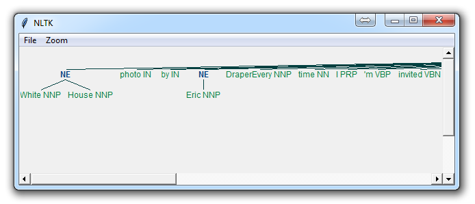
如果你設置了`binary = False`,結果為:
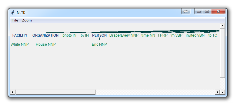
你可以馬上看到一些事情。 當`binary`是假的時候,它也選取了同樣的東西,但是把`White House`這樣的術語分解成`White`和`House`,就好像它們是不同的,而我們可以在`binary = True`的選項中看到,命名實體的識別 說`White House`是相同命名實體的一部分,這是正確的。
根據你的目標,你可以使用`binary `選項。 如果你的`binary `為`false`,這里是你可以得到的,命名實體的類型:
```
NE Type and Examples
ORGANIZATION - Georgia-Pacific Corp., WHO
PERSON - Eddy Bonte, President Obama
LOCATION - Murray River, Mount Everest
DATE - June, 2008-06-29
TIME - two fifty a m, 1:30 p.m.
MONEY - 175 million Canadian Dollars, GBP 10.40
PERCENT - twenty pct, 18.75 %
FACILITY - Washington Monument, Stonehenge
GPE - South East Asia, Midlothian
```
無論哪種方式,你可能會發現,你需要做更多的工作才能做到恰到好處,但是這個功能非常強大。
在接下來的教程中,我們將討論類似于詞干提取的東西,叫做“詞形還原”(lemmatizing)。
## 八、NLTK 詞形還原
與詞干提權非常類似的操作稱為詞形還原。 這兩者之間的主要區別是,你之前看到了,詞干提權經常可能創造出不存在的詞匯,而詞形是實際的詞匯。
所以,你的詞干,也就是你最終得到的詞,不是你可以在字典中查找的東西,但你可以查找一個詞形。
有時你最后會得到非常相似的詞語,但有時候,你會得到完全不同的詞語。 我們來看一些例子。
```py
from nltk.stem import WordNetLemmatizer
lemmatizer = WordNetLemmatizer()
print(lemmatizer.lemmatize("cats"))
print(lemmatizer.lemmatize("cacti"))
print(lemmatizer.lemmatize("geese"))
print(lemmatizer.lemmatize("rocks"))
print(lemmatizer.lemmatize("python"))
print(lemmatizer.lemmatize("better", pos="a"))
print(lemmatizer.lemmatize("best", pos="a"))
print(lemmatizer.lemmatize("run"))
print(lemmatizer.lemmatize("run",'v'))
```
在這里,我們有一些我們使用的詞的詞形的例子。 唯一要注意的是,`lemmatize `接受詞性參數`pos`。 如果沒有提供,默認是“名詞”。 這意味著,它將嘗試找到最接近的名詞,這可能會給你造成麻煩。 如果你使用詞形還原,請記住!
在接下來的教程中,我們將深入模塊附帶的 NTLK 語料庫,查看所有優秀文檔,他們在那里等待著我們。
## 九、 NLTK 語料庫
在本教程的這一部分,我想花一點時間來深入我們全部下載的語料庫! NLTK 語料庫是各種自然語言數據集,絕對值得一看。
NLTK 語料庫中的幾乎所有文件都遵循相同的規則,通過使用 NLTK 模塊來訪問它們,但是它們沒什么神奇的。 這些文件大部分都是純文本文件,其中一些是 XML 文件,另一些是其他格式文件,但都可以通過手動或模塊和 Python 訪問。 讓我們來談談手動查看它們。
根據你的安裝,你的`nltk_data`目錄可能隱藏在多個位置。 為了找出它的位置,請轉到你的 Python 目錄,也就是 NLTK 模塊所在的位置。 如果你不知道在哪里,請使用以下代碼:
```py
import nltk
print(nltk.__file__)
```
運行它,輸出將是 NLTK 模塊`__init__.py`的位置。 進入 NLTK 目錄,然后查找`data.py`文件。
代碼的重要部分是:
```py
if sys.platform.startswith('win'):
# Common locations on Windows:
path += [
str(r'C:\nltk_data'), str(r'D:\nltk_data'), str(r'E:\nltk_data'),
os.path.join(sys.prefix, str('nltk_data')),
os.path.join(sys.prefix, str('lib'), str('nltk_data')),
os.path.join(os.environ.get(str('APPDATA'), str('C:\\')), str('nltk_data'))
]
else:
# Common locations on UNIX & OS X:
path += [
str('/usr/share/nltk_data'),
str('/usr/local/share/nltk_data'),
str('/usr/lib/nltk_data'),
str('/usr/local/lib/nltk_data')
]
```
在那里,你可以看到`nltk_data`的各種可能的目錄。 如果你在 Windows 上,它很可能是在你的`appdata`中,在本地目錄中。 為此,你需要打開你的文件瀏覽器,到頂部,然后輸入`%appdata%`。
接下來點擊`roaming`,然后找到`nltk_data`目錄。 在那里,你將找到你的語料庫文件。 完整的路徑是這樣的:
```
C:\Users\yourname\AppData\Roaming\nltk_data\corpora
```
在這里,你有所有可用的語料庫,包括書籍,聊天記錄,電影評論等等。
現在,我們將討論通過 NLTK 訪問這些文檔。 正如你所看到的,這些主要是文本文檔,所以你可以使用普通的 Python 代碼來打開和閱讀文檔。 也就是說,NLTK 模塊有一些很好的處理語料庫的方法,所以你可能會發現使用他們的方法是實用的。 下面是我們打開“古騰堡圣經”,并閱讀前幾行的例子:
```py
from nltk.tokenize import sent_tokenize, PunktSentenceTokenizer
from nltk.corpus import gutenberg
# sample text
sample = gutenberg.raw("bible-kjv.txt")
tok = sent_tokenize(sample)
for x in range(5):
print(tok[x])
```
其中一個更高級的數據集是`wordnet`。 Wordnet 是一個單詞,定義,他們使用的例子,同義詞,反義詞,等等的集合。 接下來我們將深入使用 wordnet。
## 十、 NLTK 和 Wordnet
WordNet 是英語的詞匯數據庫,由普林斯頓創建,是 NLTK 語料庫的一部分。
你可以一起使用 WordNet 和 NLTK 模塊來查找單詞含義,同義詞,反義詞等。 我們來介紹一些例子。
首先,你將需要導入`wordnet`:
```py
from nltk.corpus import wordnet
```
之后我們打算使用單詞`program`來尋找同義詞:
```py
syns = wordnet.synsets("program")
```
一個同義詞的例子:
```py
print(syns[0].name())
# plan.n.01
```
只是單詞:
```py
print(syns[0].lemmas()[0].name())
# plan
```
第一個同義詞的定義:
```py
print(syns[0].definition())
# a series of steps to be carried out or goals to be accomplished
```
單詞的使用示例:
```py
print(syns[0].examples())
# ['they drew up a six-step plan', 'they discussed plans for a new bond issue']
```
接下來,我們如何辨別一個詞的同義詞和反義詞? 這些詞形是同義詞,然后你可以使用`.antonyms`找到詞形的反義詞。 因此,我們可以填充一些列表,如:
```py
synonyms = []
antonyms = []
for syn in wordnet.synsets("good"):
for l in syn.lemmas():
synonyms.append(l.name())
if l.antonyms():
antonyms.append(l.antonyms()[0].name())
print(set(synonyms))
print(set(antonyms))
'''
{'beneficial', 'just', 'upright', 'thoroughly', 'in_force', 'well', 'skilful', 'skillful', 'sound', 'unspoiled', 'expert', 'proficient', 'in_effect', 'honorable', 'adept', 'secure', 'commodity', 'estimable', 'soundly', 'right', 'respectable', 'good', 'serious', 'ripe', 'salutary', 'dear', 'practiced', 'goodness', 'safe', 'effective', 'unspoilt', 'dependable', 'undecomposed', 'honest', 'full', 'near', 'trade_good'} {'evil', 'evilness', 'bad', 'badness', 'ill'}
'''
```
你可以看到,我們的同義詞比反義詞更多,因為我們只是查找了第一個詞形的反義詞,但是你可以很容易地平衡這個,通過也為`bad`這個詞執行完全相同的過程。
接下來,我們還可以很容易地使用 WordNet 來比較兩個詞的相似性和他們的時態,把 Wu 和 Palmer 方法結合起來用于語義相關性。
我們來比較名詞`ship`和`boat`:
```py
w1 = wordnet.synset('ship.n.01')
w2 = wordnet.synset('boat.n.01')
print(w1.wup_similarity(w2))
# 0.9090909090909091
w1 = wordnet.synset('ship.n.01')
w2 = wordnet.synset('car.n.01')
print(w1.wup_similarity(w2))
# 0.6956521739130435
w1 = wordnet.synset('ship.n.01')
w2 = wordnet.synset('cat.n.01')
print(w1.wup_similarity(w2))
# 0.38095238095238093
```
接下來,我們將討論一些問題并開始討論文本分類的主題。
## 十一、NLTK 文本分類
現在我們熟悉 NLTK 了,我們來嘗試處理文本分類。 文本分類的目標可能相當寬泛。 也許我們試圖將文本分類為政治或軍事。 也許我們試圖按照作者的性別來分類。 一個相當受歡迎的文本分類任務是,將文本的正文識別為垃圾郵件或非垃圾郵件,例如電子郵件過濾器。 在我們的例子中,我們將嘗試創建一個情感分析算法。
為此,我們首先嘗試使用屬于 NLTK 語料庫的電影評論數據庫。 從那里,我們將嘗試使用詞匯作為“特征”,這是“正面”或“負面”電影評論的一部分。 NLTK 語料庫`movie_reviews`數據集擁有評論,他們被標記為正面或負面。 這意味著我們可以訓練和測試這些數據。 首先,讓我們來預處理我們的數據。
```py
import nltk
import random
from nltk.corpus import movie_reviews
documents = [(list(movie_reviews.words(fileid)), category)
for category in movie_reviews.categories()
for fileid in movie_reviews.fileids(category)]
random.shuffle(documents)
print(documents[1])
all_words = []
for w in movie_reviews.words():
all_words.append(w.lower())
all_words = nltk.FreqDist(all_words)
print(all_words.most_common(15))
print(all_words["stupid"])
```
運行此腳本可能需要一些時間,因為電影評論數據集有點大。 我們來介紹一下這里發生的事情。
導入我們想要的數據集后,你會看到:
```py
documents = [(list(movie_reviews.words(fileid)), category)
for category in movie_reviews.categories()
for fileid in movie_reviews.fileids(category)]
```
基本上,用簡單的英文,上面的代碼被翻譯成:在每個類別(我們有正向和獨享),選取所有的文件 ID(每個評論有自己的 ID),然后對文件 ID存儲`word_tokenized`版本(單詞列表),后面是一個大列表中的正面或負面標簽。
接下來,我們用`random `來打亂我們的文件。這是因為我們將要進行訓練和測試。如果我們把他們按序排列,我們可能會訓練所有的負面評論,和一些正面評論,然后在所有正面評論上測試。我們不想這樣,所以我們打亂了數據。
然后,為了你能看到你正在使用的數據,我們打印出`documents[1]`,這是一個大列表,其中第一個元素是一列單詞,第二個元素是`pos`或`neg`標簽。
接下來,我們要收集我們找到的所有單詞,所以我們可以有一個巨大的典型單詞列表。從這里,我們可以執行一個頻率分布,然后找出最常見的單詞。正如你所看到的,最受歡迎的“詞語”其實就是標點符號,`the`,`a`等等,但是很快我們就會得到有效詞匯。我們打算存儲幾千個最流行的單詞,所以這不應該是一個問題。
```py
print(all_words.most_common(15))
```
以上給出了15個最常用的單詞。 你也可以通過下面的步驟找出一個單詞的出現次數:
```py
print(all_words["stupid"])
```
接下來,我們開始將我們的單詞,儲存為正面或負面的電影評論的特征。
## 十二、使用 NLTK 將單詞轉換為特征
在本教程中,我們在以前的視頻基礎上構建,并編撰正面評論和負面評論中的單詞的特征列表,來看到正面或負面評論中特定類型單詞的趨勢。
最初,我們的代碼:
```py
import nltk
import random
from nltk.corpus import movie_reviews
documents = [(list(movie_reviews.words(fileid)), category)
for category in movie_reviews.categories()
for fileid in movie_reviews.fileids(category)]
random.shuffle(documents)
all_words = []
for w in movie_reviews.words():
all_words.append(w.lower())
all_words = nltk.FreqDist(all_words)
word_features = list(all_words.keys())[:3000]
```
幾乎和以前一樣,只是現在有一個新的變量,`word_features`,它包含了前 3000 個最常用的單詞。 接下來,我們將建立一個簡單的函數,在我們的正面和負面的文檔中找到這些前 3000 個單詞,將他們的存在標記為是或否:
```py
def find_features(document):
words = set(document)
features = {}
for w in word_features:
features[w] = (w in words)
return features
```
下面,我們可以打印出特征集:
```py
print((find_features(movie_reviews.words('neg/cv000_29416.txt'))))
```
之后我們可以為我們所有的文檔做這件事情,通過做下列事情,保存特征存在性布爾值,以及它們各自的正面或負面的類別:
```py
featuresets = [(find_features(rev), category) for (rev, category) in documents]
```
真棒,現在我們有了特征和標簽,接下來是什么? 通常,下一步是繼續并訓練算法,然后對其進行測試。 所以,讓我們繼續這樣做,從下一個教程中的樸素貝葉斯分類器開始!
## 十三、NLTK 樸素貝葉斯分類器
現在是時候選擇一個算法,將我們的數據分成訓練和測試集,然后啟動!我們首先要使用的算法是樸素貝葉斯分類器。這是一個非常受歡迎的文本分類算法,所以我們只能先試一試。然而,在我們可以訓練和測試我們的算法之前,我們需要先把數據分解成訓練集和測試集。
你可以訓練和測試同一個數據集,但是這會給你帶來一些嚴重的偏差問題,所以你不應該訓練和測試完全相同的數據。為此,由于我們已經打亂了數據集,因此我們將首先將包含正面和負面評論的 1900 個亂序評論作為訓練集。然后,我們可以在最后的 100 個上測試,看看我們有多準確。
這被稱為監督機器學習,因為我們正在向機器展示數據,并告訴它“這個數據是正面的”,或者“這個數據是負面的”。然后,在完成訓練之后,我們向機器展示一些新的數據,并根據我們之前教過計算機的內容詢問計算機,計算機認為新數據的類別是什么。
我們可以用以下方式分割數據:
```py
# set that we'll train our classifier with
training_set = featuresets[:1900]
# set that we'll test against.
testing_set = featuresets[1900:]
```
下面,我們可以定義并訓練我們的分類器:
```py
classifier = nltk.NaiveBayesClassifier.train(training_set)
```
首先,我們只是簡單調用樸素貝葉斯分類器,然后在一行中使用`.train()`進行訓練。
足夠簡單,現在它得到了訓練。 接下來,我們可以測試它:
```py
print("Classifier accuracy percent:",(nltk.classify.accuracy(classifier, testing_set))*100)
```
砰,你得到了你的答案。 如果你錯過了,我們可以“測試”數據的原因是,我們仍然有正確的答案。 因此,在測試中,我們向計算機展示數據,而不提供正確的答案。 如果它正確猜測我們所知的答案,那么計算機是正確的。 考慮到我們所做的打亂,你和我可能準確度不同,但你應該看到準確度平均為 60-75%。
接下來,我們可以進一步了解正面或負面評論中最有價值的詞匯:
```py
classifier.show_most_informative_features(15)
```
這對于每個人都不一樣,但是你應該看到這樣的東西:
```
Most Informative Features
insulting = True neg : pos = 10.6 : 1.0
ludicrous = True neg : pos = 10.1 : 1.0
winslet = True pos : neg = 9.0 : 1.0
detract = True pos : neg = 8.4 : 1.0
breathtaking = True pos : neg = 8.1 : 1.0
silverstone = True neg : pos = 7.6 : 1.0
excruciatingly = True neg : pos = 7.6 : 1.0
warns = True pos : neg = 7.0 : 1.0
tracy = True pos : neg = 7.0 : 1.0
insipid = True neg : pos = 7.0 : 1.0
freddie = True neg : pos = 7.0 : 1.0
damon = True pos : neg = 5.9 : 1.0
debate = True pos : neg = 5.9 : 1.0
ordered = True pos : neg = 5.8 : 1.0
lang = True pos : neg = 5.7 : 1.0
```
這個告訴你的是,每一個詞的負面到正面的出現幾率,或相反。 因此,在這里,我們可以看到,負面評論中的`insulting`一詞比正面評論多出現 10.6 倍。`Ludicrous`是 10.1。
現在,讓我們假設,你完全滿意你的結果,你想要繼續,也許使用這個分類器來預測現在的事情。 訓練分類器,并且每當你需要使用分類器時,都要重新訓練,是非常不切實際的。 因此,你可以使用`pickle`模塊保存分類器。 我們接下來做。
## 十四、使用 NLTK 保存分類器
訓練分類器和機器學習算法可能需要很長時間,特別是如果你在更大的數據集上訓練。 我們的其實很小。 你可以想象,每次你想開始使用分類器的時候,都要訓練分類器嗎? 這么恐怖! 相反,我們可以使用`pickle`模塊,并序列化我們的分類器對象,這樣我們所需要做的就是簡單加載該文件。
那么,我們該怎么做呢? 第一步是保存對象。 為此,首先需要在腳本的頂部導入`pickle`,然后在使用`.train()`分類器進行訓練后,可以調用以下幾行:
```py
save_classifier = open("naivebayes.pickle","wb")
pickle.dump(classifier, save_classifier)
save_classifier.close()
```
這打開了一個`pickle`文件,準備按字節寫入一些數據。 然后,我們使用`pickle.dump()`來轉儲數據。 `pickle.dump()`的第一個參數是你寫入的東西,第二個參數是你寫入它的地方。
之后,我們按照我們的要求關閉文件,這就是說,我們現在在腳本的目錄中保存了一個`pickle`或序列化的對象!
接下來,我們如何開始使用這個分類器? `.pickle`文件是序列化的對象,我們現在需要做的就是將其讀入內存,這與讀取任何其他普通文件一樣簡單。 這樣做:
```py
classifier_f = open("naivebayes.pickle", "rb")
classifier = pickle.load(classifier_f)
classifier_f.close()
```
在這里,我們執行了非常相似的過程。 我們打開文件來讀取字節。 然后,我們使用`pickle.load()`來加載文件,并將數據保存到分類器變量中。 然后我們關閉文件,就是這樣。 我們現在有了和以前一樣的分類器對象!
現在,我們可以使用這個對象,每當我們想用它來分類時,我們不再需要訓練我們的分類器。
雖然這一切都很好,但是我們可能不太滿意我們所獲得的 60-75% 的準確度。 其他分類器呢? 其實,有很多分類器,但我們需要 scikit-learn(sklearn)模塊。 幸運的是,NLTK 的員工認識到將 sklearn 模塊納入 NLTK 的價值,他們為我們構建了一個小 API。 這就是我們將在下一個教程中做的事情。
## 十五、NLTK 和 Sklearn
現在我們已經看到,使用分類器是多么容易,現在我們想嘗試更多東西! Python 的最好的模塊是 Scikit-learn(sklearn)模塊。
如果你想了解 Scikit-learn 模塊的更多信息,我有一些關于 Scikit-Learn 機器學習的教程。
幸運的是,對于我們來說,NLTK 背后的人們更看重將 sklearn 模塊納入NLTK分類器方法的價值。 就這樣,他們創建了各種`SklearnClassifier` API。 要使用它,你只需要像下面這樣導入它:
```py
from nltk.classify.scikitlearn import SklearnClassifier
```
從這里開始,你可以使用任何`sklearn`分類器。 例如,讓我們引入更多的樸素貝葉斯算法的變體:
```py
from sklearn.naive_bayes import MultinomialNB,BernoulliNB
```
之后,如何使用它們?結果是,這非常簡單。
```py
MNB_classifier = SklearnClassifier(MultinomialNB())
MNB_classifier.train(training_set)
print("MultinomialNB accuracy percent:",nltk.classify.accuracy(MNB_classifier, testing_set))
BNB_classifier = SklearnClassifier(BernoulliNB())
BNB_classifier.train(training_set)
print("BernoulliNB accuracy percent:",nltk.classify.accuracy(BNB_classifier, testing_set))
```
就是這么簡單。讓我們引入更多東西:
```py
from sklearn.linear_model import LogisticRegression,SGDClassifier
from sklearn.svm import SVC, LinearSVC, NuSVC
```
現在,我們所有分類器應該是這樣:
```py
print("Original Naive Bayes Algo accuracy percent:", (nltk.classify.accuracy(classifier, testing_set))*100)
classifier.show_most_informative_features(15)
MNB_classifier = SklearnClassifier(MultinomialNB())
MNB_classifier.train(training_set)
print("MNB_classifier accuracy percent:", (nltk.classify.accuracy(MNB_classifier, testing_set))*100)
BernoulliNB_classifier = SklearnClassifier(BernoulliNB())
BernoulliNB_classifier.train(training_set)
print("BernoulliNB_classifier accuracy percent:", (nltk.classify.accuracy(BernoulliNB_classifier, testing_set))*100)
LogisticRegression_classifier = SklearnClassifier(LogisticRegression())
LogisticRegression_classifier.train(training_set)
print("LogisticRegression_classifier accuracy percent:", (nltk.classify.accuracy(LogisticRegression_classifier, testing_set))*100)
SGDClassifier_classifier = SklearnClassifier(SGDClassifier())
SGDClassifier_classifier.train(training_set)
print("SGDClassifier_classifier accuracy percent:", (nltk.classify.accuracy(SGDClassifier_classifier, testing_set))*100)
SVC_classifier = SklearnClassifier(SVC())
SVC_classifier.train(training_set)
print("SVC_classifier accuracy percent:", (nltk.classify.accuracy(SVC_classifier, testing_set))*100)
LinearSVC_classifier = SklearnClassifier(LinearSVC())
LinearSVC_classifier.train(training_set)
print("LinearSVC_classifier accuracy percent:", (nltk.classify.accuracy(LinearSVC_classifier, testing_set))*100)
NuSVC_classifier = SklearnClassifier(NuSVC())
NuSVC_classifier.train(training_set)
print("NuSVC_classifier accuracy percent:", (nltk.classify.accuracy(NuSVC_classifier, testing_set))*100)
```
運行它的結果應該是這樣:
```
Original Naive Bayes Algo accuracy percent: 63.0
Most Informative Features
thematic = True pos : neg = 9.1 : 1.0
secondly = True pos : neg = 8.5 : 1.0
narrates = True pos : neg = 7.8 : 1.0
rounded = True pos : neg = 7.1 : 1.0
supreme = True pos : neg = 7.1 : 1.0
layered = True pos : neg = 7.1 : 1.0
crappy = True neg : pos = 6.9 : 1.0
uplifting = True pos : neg = 6.2 : 1.0
ugh = True neg : pos = 5.3 : 1.0
mamet = True pos : neg = 5.1 : 1.0
gaining = True pos : neg = 5.1 : 1.0
wanda = True neg : pos = 4.9 : 1.0
onset = True neg : pos = 4.9 : 1.0
fantastic = True pos : neg = 4.5 : 1.0
kentucky = True pos : neg = 4.4 : 1.0
MNB_classifier accuracy percent: 66.0
BernoulliNB_classifier accuracy percent: 72.0
LogisticRegression_classifier accuracy percent: 64.0
SGDClassifier_classifier accuracy percent: 61.0
SVC_classifier accuracy percent: 45.0
LinearSVC_classifier accuracy percent: 68.0
NuSVC_classifier accuracy percent: 59.0
```
所以,我們可以看到,SVC 的錯誤比正確更常見,所以我們可能應該丟棄它。 但是呢? 接下來我們可以嘗試一次使用所有這些算法。 一個算法的算法! 為此,我們可以創建另一個分類器,并根據其他算法的結果來生成分類器的結果。 有點像投票系統,所以我們只需要奇數數量的算法。 這就是我們將在下一個教程中討論的內容。
## 十六、使用 NLTK 組合算法
現在我們知道如何使用一堆算法分類器,就像糖果島上的一個孩子,告訴他們只能選擇一個,我們可能會發現很難只選擇一個分類器。 好消息是,你不必這樣! 組合分類器算法是一種常用的技術,通過創建一種投票系統來實現,每個算法擁有一票,選擇得票最多分類。
為此,我們希望我們的新分類器的工作方式像典型的 NLTK 分類器,并擁有所有方法。 很簡單,使用面向對象編程,我們可以確保從 NLTK 分類器類繼承。 為此,我們將導入它:
```py
from nltk.classify import ClassifierI
from statistics import mode
```
我們也導入`mode`(眾數),因為這將是我們選擇最大計數的方法。
現在,我們來建立我們的分類器類:
```py
class VoteClassifier(ClassifierI):
def __init__(self, *classifiers):
self._classifiers = classifiers
```
我們把我們的類叫做`VoteClassifier`,我們繼承了 NLTK 的`ClassifierI`。 接下來,我們將傳遞給我們的類的分類器列表賦給`self._classifiers`。
接下來,我們要繼續創建我們自己的分類方法。 我們打算把它稱為`.classify`,以便我們可以稍后調用`.classify`,就像傳統的 NLTK 分類器那樣。
```py
def classify(self, features):
votes = []
for c in self._classifiers:
v = c.classify(features)
votes.append(v)
return mode(votes)
```
很簡單,我們在這里所做的就是,遍歷我們的分類器對象列表。 然后,對于每一個,我們要求它基于特征分類。 分類被視為投票。 遍歷完成后,我們返回`mode(votes)`,這只是返回投票的眾數。
這是我們真正需要的,但是我認為另一個參數,置信度是有用的。 由于我們有了投票算法,所以我們也可以統計支持和反對票數,并稱之為“置信度”。 例如,3/5 票的置信度弱于 5/5 票。 因此,我們可以從字面上返回投票比例,作為一種置信度指標。 這是我們的置信度方法:
```py
def confidence(self, features):
votes = []
for c in self._classifiers:
v = c.classify(features)
votes.append(v)
choice_votes = votes.count(mode(votes))
conf = choice_votes / len(votes)
return conf
```
現在,讓我們把東西放到一起:
```py
import nltk
import random
from nltk.corpus import movie_reviews
from nltk.classify.scikitlearn import SklearnClassifier
import pickle
from sklearn.naive_bayes import MultinomialNB, BernoulliNB
from sklearn.linear_model import LogisticRegression, SGDClassifier
from sklearn.svm import SVC, LinearSVC, NuSVC
from nltk.classify import ClassifierI
from statistics import mode
class VoteClassifier(ClassifierI):
def __init__(self, *classifiers):
self._classifiers = classifiers
def classify(self, features):
votes = []
for c in self._classifiers:
v = c.classify(features)
votes.append(v)
return mode(votes)
def confidence(self, features):
votes = []
for c in self._classifiers:
v = c.classify(features)
votes.append(v)
choice_votes = votes.count(mode(votes))
conf = choice_votes / len(votes)
return conf
documents = [(list(movie_reviews.words(fileid)), category)
for category in movie_reviews.categories()
for fileid in movie_reviews.fileids(category)]
random.shuffle(documents)
all_words = []
for w in movie_reviews.words():
all_words.append(w.lower())
all_words = nltk.FreqDist(all_words)
word_features = list(all_words.keys())[:3000]
def find_features(document):
words = set(document)
features = {}
for w in word_features:
features[w] = (w in words)
return features
#print((find_features(movie_reviews.words('neg/cv000_29416.txt'))))
featuresets = [(find_features(rev), category) for (rev, category) in documents]
training_set = featuresets[:1900]
testing_set = featuresets[1900:]
#classifier = nltk.NaiveBayesClassifier.train(training_set)
classifier_f = open("naivebayes.pickle","rb")
classifier = pickle.load(classifier_f)
classifier_f.close()
print("Original Naive Bayes Algo accuracy percent:", (nltk.classify.accuracy(classifier, testing_set))*100)
classifier.show_most_informative_features(15)
MNB_classifier = SklearnClassifier(MultinomialNB())
MNB_classifier.train(training_set)
print("MNB_classifier accuracy percent:", (nltk.classify.accuracy(MNB_classifier, testing_set))*100)
BernoulliNB_classifier = SklearnClassifier(BernoulliNB())
BernoulliNB_classifier.train(training_set)
print("BernoulliNB_classifier accuracy percent:", (nltk.classify.accuracy(BernoulliNB_classifier, testing_set))*100)
LogisticRegression_classifier = SklearnClassifier(LogisticRegression())
LogisticRegression_classifier.train(training_set)
print("LogisticRegression_classifier accuracy percent:", (nltk.classify.accuracy(LogisticRegression_classifier, testing_set))*100)
SGDClassifier_classifier = SklearnClassifier(SGDClassifier())
SGDClassifier_classifier.train(training_set)
print("SGDClassifier_classifier accuracy percent:", (nltk.classify.accuracy(SGDClassifier_classifier, testing_set))*100)
##SVC_classifier = SklearnClassifier(SVC())
##SVC_classifier.train(training_set)
##print("SVC_classifier accuracy percent:", (nltk.classify.accuracy(SVC_classifier, testing_set))*100)
LinearSVC_classifier = SklearnClassifier(LinearSVC())
LinearSVC_classifier.train(training_set)
print("LinearSVC_classifier accuracy percent:", (nltk.classify.accuracy(LinearSVC_classifier, testing_set))*100)
NuSVC_classifier = SklearnClassifier(NuSVC())
NuSVC_classifier.train(training_set)
print("NuSVC_classifier accuracy percent:", (nltk.classify.accuracy(NuSVC_classifier, testing_set))*100)
voted_classifier = VoteClassifier(classifier,
NuSVC_classifier,
LinearSVC_classifier,
SGDClassifier_classifier,
MNB_classifier,
BernoulliNB_classifier,
LogisticRegression_classifier)
print("voted_classifier accuracy percent:", (nltk.classify.accuracy(voted_classifier, testing_set))*100)
print("Classification:", voted_classifier.classify(testing_set[0][0]), "Confidence %:",voted_classifier.confidence(testing_set[0][0])*100)
print("Classification:", voted_classifier.classify(testing_set[1][0]), "Confidence %:",voted_classifier.confidence(testing_set[1][0])*100)
print("Classification:", voted_classifier.classify(testing_set[2][0]), "Confidence %:",voted_classifier.confidence(testing_set[2][0])*100)
print("Classification:", voted_classifier.classify(testing_set[3][0]), "Confidence %:",voted_classifier.confidence(testing_set[3][0])*100)
print("Classification:", voted_classifier.classify(testing_set[4][0]), "Confidence %:",voted_classifier.confidence(testing_set[4][0])*100)
print("Classification:", voted_classifier.classify(testing_set[5][0]), "Confidence %:",voted_classifier.confidence(testing_set[5][0])*100)
```
所以到了最后,我們對文本運行一些分類器示例。我們所有輸出:
```
Original Naive Bayes Algo accuracy percent: 66.0
Most Informative Features
thematic = True pos : neg = 9.1 : 1.0
secondly = True pos : neg = 8.5 : 1.0
narrates = True pos : neg = 7.8 : 1.0
layered = True pos : neg = 7.1 : 1.0
rounded = True pos : neg = 7.1 : 1.0
supreme = True pos : neg = 7.1 : 1.0
crappy = True neg : pos = 6.9 : 1.0
uplifting = True pos : neg = 6.2 : 1.0
ugh = True neg : pos = 5.3 : 1.0
gaining = True pos : neg = 5.1 : 1.0
mamet = True pos : neg = 5.1 : 1.0
wanda = True neg : pos = 4.9 : 1.0
onset = True neg : pos = 4.9 : 1.0
fantastic = True pos : neg = 4.5 : 1.0
milos = True pos : neg = 4.4 : 1.0
MNB_classifier accuracy percent: 67.0
BernoulliNB_classifier accuracy percent: 67.0
LogisticRegression_classifier accuracy percent: 68.0
SGDClassifier_classifier accuracy percent: 57.99999999999999
LinearSVC_classifier accuracy percent: 67.0
NuSVC_classifier accuracy percent: 65.0
voted_classifier accuracy percent: 65.0
Classification: neg Confidence %: 100.0
Classification: pos Confidence %: 57.14285714285714
Classification: neg Confidence %: 57.14285714285714
Classification: neg Confidence %: 57.14285714285714
Classification: pos Confidence %: 57.14285714285714
Classification: pos Confidence %: 85.71428571428571
```
## 十七、使用 NLTK 調查偏差
在本教程中,我們將討論一些問題。最主要的問題是我們有一個相當有偏差的算法。你可以通過注釋掉文檔的打亂,然后使用前 1900 個進行訓練,并留下最后的 100 個(所有正面)評論來測試它。測試它,你會發現你的準確性很差。
相反,你可以使用前 100 個數據進行測試,所有的數據都是負面的,并且使用后 1900 個訓練。在這里你會發現準確度非常高。這是一個不好的跡象。這可能意味著很多東西,我們有很多選擇來解決它。
也就是說,我們所考慮的項目建議我們繼續,并使用不同的數據集,所以我們會這樣做。最后,我們會發現這個新的數據集仍然存在一些偏差,那就是它更經常選擇負面的東西。原因是負面評論的負面往往比正面評論的正面程度更大。這個可以用一些簡單的加權來完成,但是它也可以變得很復雜。也許是另一天的教程。現在,我們要抓取一個新的數據集,我們將在下一個教程中討論這個數據集。
## 十八、使用 NLTK 改善情感分析的訓練數據
所以現在是時候在新的數據集上訓練了。 我們的目標是分析 Twitter 的情緒,所以我們希望數據集的每個正面和負面語句都有點短。 恰好我有 5300+ 個正面和 5300 + 個負面電影評論,這是短得多的數據集。 我們應該能從更大的訓練集中獲得更多的準確性,并且把 Twitter 的推文擬合得更好。
我在這里托管了這兩個文件,你可以通過[下載簡短的評論](https://pythonprogramming.net/static/downloads/short_reviews/)來找到它們。 將這些文件保存為`positive.txt`和`negative.txt`。
現在,我們可以像以前一樣建立新的數據集。 需要改變什么呢?
我們需要一種新的方法來創建我們的“文檔”變量,然后我們還需要一種新的方法來創建`all_words`變量。 真的沒問題,我是這么做的:
```py
short_pos = open("short_reviews/positive.txt","r").read()
short_neg = open("short_reviews/negative.txt","r").read()
documents = []
for r in short_pos.split('\n'):
documents.append( (r, "pos") )
for r in short_neg.split('\n'):
documents.append( (r, "neg") )
all_words = []
short_pos_words = word_tokenize(short_pos)
short_neg_words = word_tokenize(short_neg)
for w in short_pos_words:
all_words.append(w.lower())
for w in short_neg_words:
all_words.append(w.lower())
all_words = nltk.FreqDist(all_words)
```
接下來,我們還需要調整我們的特征查找功能,主要是按照文檔中的單詞進行標記,因為我們的新樣本沒有漂亮的`.words()`特征。 我繼續并增加了最常見的詞語:
```py
word_features = list(all_words.keys())[:5000]
def find_features(document):
words = word_tokenize(document)
features = {}
for w in word_features:
features[w] = (w in words)
return features
featuresets = [(find_features(rev), category) for (rev, category) in documents]
random.shuffle(featuresets)
```
除此之外,其余的都是一樣的。 這是完整的腳本,以防萬一你或我錯過了一些東西:
這個過程需要一段時間..你可能想要干些別的。 我花了大約 30-40 分鐘來全部運行完成,而我在 i7 3930k 上運行它。 在我寫這篇文章的時候(2015),一般處理器可能需要幾個小時。 不過這是一次性的過程。
```py
import nltk
import random
from nltk.corpus import movie_reviews
from nltk.classify.scikitlearn import SklearnClassifier
import pickle
from sklearn.naive_bayes import MultinomialNB, BernoulliNB
from sklearn.linear_model import LogisticRegression, SGDClassifier
from sklearn.svm import SVC, LinearSVC, NuSVC
from nltk.classify import ClassifierI
from statistics import mode
from nltk.tokenize import word_tokenize
class VoteClassifier(ClassifierI):
def __init__(self, *classifiers):
self._classifiers = classifiers
def classify(self, features):
votes = []
for c in self._classifiers:
v = c.classify(features)
votes.append(v)
return mode(votes)
def confidence(self, features):
votes = []
for c in self._classifiers:
v = c.classify(features)
votes.append(v)
choice_votes = votes.count(mode(votes))
conf = choice_votes / len(votes)
return conf
short_pos = open("short_reviews/positive.txt","r").read()
short_neg = open("short_reviews/negative.txt","r").read()
documents = []
for r in short_pos.split('\n'):
documents.append( (r, "pos") )
for r in short_neg.split('\n'):
documents.append( (r, "neg") )
all_words = []
short_pos_words = word_tokenize(short_pos)
short_neg_words = word_tokenize(short_neg)
for w in short_pos_words:
all_words.append(w.lower())
for w in short_neg_words:
all_words.append(w.lower())
all_words = nltk.FreqDist(all_words)
word_features = list(all_words.keys())[:5000]
def find_features(document):
words = word_tokenize(document)
features = {}
for w in word_features:
features[w] = (w in words)
return features
#print((find_features(movie_reviews.words('neg/cv000_29416.txt'))))
featuresets = [(find_features(rev), category) for (rev, category) in documents]
random.shuffle(featuresets)
# positive data example:
training_set = featuresets[:10000]
testing_set = featuresets[10000:]
##
### negative data example:
##training_set = featuresets[100:]
##testing_set = featuresets[:100]
classifier = nltk.NaiveBayesClassifier.train(training_set)
print("Original Naive Bayes Algo accuracy percent:", (nltk.classify.accuracy(classifier, testing_set))*100)
classifier.show_most_informative_features(15)
MNB_classifier = SklearnClassifier(MultinomialNB())
MNB_classifier.train(training_set)
print("MNB_classifier accuracy percent:", (nltk.classify.accuracy(MNB_classifier, testing_set))*100)
BernoulliNB_classifier = SklearnClassifier(BernoulliNB())
BernoulliNB_classifier.train(training_set)
print("BernoulliNB_classifier accuracy percent:", (nltk.classify.accuracy(BernoulliNB_classifier, testing_set))*100)
LogisticRegression_classifier = SklearnClassifier(LogisticRegression())
LogisticRegression_classifier.train(training_set)
print("LogisticRegression_classifier accuracy percent:", (nltk.classify.accuracy(LogisticRegression_classifier, testing_set))*100)
SGDClassifier_classifier = SklearnClassifier(SGDClassifier())
SGDClassifier_classifier.train(training_set)
print("SGDClassifier_classifier accuracy percent:", (nltk.classify.accuracy(SGDClassifier_classifier, testing_set))*100)
##SVC_classifier = SklearnClassifier(SVC())
##SVC_classifier.train(training_set)
##print("SVC_classifier accuracy percent:", (nltk.classify.accuracy(SVC_classifier, testing_set))*100)
LinearSVC_classifier = SklearnClassifier(LinearSVC())
LinearSVC_classifier.train(training_set)
print("LinearSVC_classifier accuracy percent:", (nltk.classify.accuracy(LinearSVC_classifier, testing_set))*100)
NuSVC_classifier = SklearnClassifier(NuSVC())
NuSVC_classifier.train(training_set)
print("NuSVC_classifier accuracy percent:", (nltk.classify.accuracy(NuSVC_classifier, testing_set))*100)
voted_classifier = VoteClassifier(
NuSVC_classifier,
LinearSVC_classifier,
MNB_classifier,
BernoulliNB_classifier,
LogisticRegression_classifier)
print("voted_classifier accuracy percent:", (nltk.classify.accuracy(voted_classifier, testing_set))*100)
```
輸出:
```
Original Naive Bayes Algo accuracy percent: 66.26506024096386
Most Informative Features
refreshing = True pos : neg = 13.6 : 1.0
captures = True pos : neg = 11.3 : 1.0
stupid = True neg : pos = 10.7 : 1.0
tender = True pos : neg = 9.6 : 1.0
meandering = True neg : pos = 9.1 : 1.0
tv = True neg : pos = 8.6 : 1.0
low-key = True pos : neg = 8.3 : 1.0
thoughtful = True pos : neg = 8.1 : 1.0
banal = True neg : pos = 7.7 : 1.0
amateurish = True neg : pos = 7.7 : 1.0
terrific = True pos : neg = 7.6 : 1.0
record = True pos : neg = 7.6 : 1.0
captivating = True pos : neg = 7.6 : 1.0
portrait = True pos : neg = 7.4 : 1.0
culture = True pos : neg = 7.3 : 1.0
MNB_classifier accuracy percent: 65.8132530120482
BernoulliNB_classifier accuracy percent: 66.71686746987952
LogisticRegression_classifier accuracy percent: 67.16867469879519
SGDClassifier_classifier accuracy percent: 65.8132530120482
LinearSVC_classifier accuracy percent: 66.71686746987952
NuSVC_classifier accuracy percent: 60.09036144578314
voted_classifier accuracy percent: 65.66265060240963
```
是的,我敢打賭你花了一段時間,所以,在下一個教程中,我們將談論`pickle`所有東西!
## 十九、使用 NLTK 為情感分析創建模塊
有了這個新的數據集和新的分類器,我們可以繼續前進。 你可能已經注意到的,這個新的數據集需要更長的時間來訓練,因為它是一個更大的集合。 我已經向你顯示,通過`pickel`或序列化訓練出來的分類器,我們實際上可以節省大量的時間,這些分類器只是對象。
我已經向你證明了如何使用`pickel`來實現它,所以我鼓勵你嘗試自己做。 如果你需要幫助,我會粘貼完整的代碼...但要注意,自己動手!
這個過程需要一段時間..你可能想要干些別的。 我花了大約 30-40 分鐘來全部運行完成,而我在 i7 3930k 上運行它。 在我寫這篇文章的時候(2015),一般處理器可能需要幾個小時。 不過這是一次性的過程。
```py
import nltk
import random
#from nltk.corpus import movie_reviews
from nltk.classify.scikitlearn import SklearnClassifier
import pickle
from sklearn.naive_bayes import MultinomialNB, BernoulliNB
from sklearn.linear_model import LogisticRegression, SGDClassifier
from sklearn.svm import SVC, LinearSVC, NuSVC
from nltk.classify import ClassifierI
from statistics import mode
from nltk.tokenize import word_tokenize
class VoteClassifier(ClassifierI):
def __init__(self, *classifiers):
self._classifiers = classifiers
def classify(self, features):
votes = []
for c in self._classifiers:
v = c.classify(features)
votes.append(v)
return mode(votes)
def confidence(self, features):
votes = []
for c in self._classifiers:
v = c.classify(features)
votes.append(v)
choice_votes = votes.count(mode(votes))
conf = choice_votes / len(votes)
return conf
short_pos = open("short_reviews/positive.txt","r").read()
short_neg = open("short_reviews/negative.txt","r").read()
# move this up here
all_words = []
documents = []
# j is adject, r is adverb, and v is verb
#allowed_word_types = ["J","R","V"]
allowed_word_types = ["J"]
for p in short_pos.split('\n'):
documents.append( (p, "pos") )
words = word_tokenize(p)
pos = nltk.pos_tag(words)
for w in pos:
if w[1][0] in allowed_word_types:
all_words.append(w[0].lower())
for p in short_neg.split('\n'):
documents.append( (p, "neg") )
words = word_tokenize(p)
pos = nltk.pos_tag(words)
for w in pos:
if w[1][0] in allowed_word_types:
all_words.append(w[0].lower())
save_documents = open("pickled_algos/documents.pickle","wb")
pickle.dump(documents, save_documents)
save_documents.close()
all_words = nltk.FreqDist(all_words)
word_features = list(all_words.keys())[:5000]
save_word_features = open("pickled_algos/word_features5k.pickle","wb")
pickle.dump(word_features, save_word_features)
save_word_features.close()
def find_features(document):
words = word_tokenize(document)
features = {}
for w in word_features:
features[w] = (w in words)
return features
featuresets = [(find_features(rev), category) for (rev, category) in documents]
random.shuffle(featuresets)
print(len(featuresets))
testing_set = featuresets[10000:]
training_set = featuresets[:10000]
classifier = nltk.NaiveBayesClassifier.train(training_set)
print("Original Naive Bayes Algo accuracy percent:", (nltk.classify.accuracy(classifier, testing_set))*100)
classifier.show_most_informative_features(15)
###############
save_classifier = open("pickled_algos/originalnaivebayes5k.pickle","wb")
pickle.dump(classifier, save_classifier)
save_classifier.close()
MNB_classifier = SklearnClassifier(MultinomialNB())
MNB_classifier.train(training_set)
print("MNB_classifier accuracy percent:", (nltk.classify.accuracy(MNB_classifier, testing_set))*100)
save_classifier = open("pickled_algos/MNB_classifier5k.pickle","wb")
pickle.dump(MNB_classifier, save_classifier)
save_classifier.close()
BernoulliNB_classifier = SklearnClassifier(BernoulliNB())
BernoulliNB_classifier.train(training_set)
print("BernoulliNB_classifier accuracy percent:", (nltk.classify.accuracy(BernoulliNB_classifier, testing_set))*100)
save_classifier = open("pickled_algos/BernoulliNB_classifier5k.pickle","wb")
pickle.dump(BernoulliNB_classifier, save_classifier)
save_classifier.close()
LogisticRegression_classifier = SklearnClassifier(LogisticRegression())
LogisticRegression_classifier.train(training_set)
print("LogisticRegression_classifier accuracy percent:", (nltk.classify.accuracy(LogisticRegression_classifier, testing_set))*100)
save_classifier = open("pickled_algos/LogisticRegression_classifier5k.pickle","wb")
pickle.dump(LogisticRegression_classifier, save_classifier)
save_classifier.close()
LinearSVC_classifier = SklearnClassifier(LinearSVC())
LinearSVC_classifier.train(training_set)
print("LinearSVC_classifier accuracy percent:", (nltk.classify.accuracy(LinearSVC_classifier, testing_set))*100)
save_classifier = open("pickled_algos/LinearSVC_classifier5k.pickle","wb")
pickle.dump(LinearSVC_classifier, save_classifier)
save_classifier.close()
##NuSVC_classifier = SklearnClassifier(NuSVC())
##NuSVC_classifier.train(training_set)
##print("NuSVC_classifier accuracy percent:", (nltk.classify.accuracy(NuSVC_classifier, testing_set))*100)
SGDC_classifier = SklearnClassifier(SGDClassifier())
SGDC_classifier.train(training_set)
print("SGDClassifier accuracy percent:",nltk.classify.accuracy(SGDC_classifier, testing_set)*100)
save_classifier = open("pickled_algos/SGDC_classifier5k.pickle","wb")
pickle.dump(SGDC_classifier, save_classifier)
save_classifier.close()
```
現在,你只需要運行一次。 如果你希望,你可以隨時運行它,但現在,你已經準備好了創建情緒分析模塊。 這是我們稱為`sentiment_mod.py`的文件:
```py
#File: sentiment_mod.py
import nltk
import random
#from nltk.corpus import movie_reviews
from nltk.classify.scikitlearn import SklearnClassifier
import pickle
from sklearn.naive_bayes import MultinomialNB, BernoulliNB
from sklearn.linear_model import LogisticRegression, SGDClassifier
from sklearn.svm import SVC, LinearSVC, NuSVC
from nltk.classify import ClassifierI
from statistics import mode
from nltk.tokenize import word_tokenize
class VoteClassifier(ClassifierI):
def __init__(self, *classifiers):
self._classifiers = classifiers
def classify(self, features):
votes = []
for c in self._classifiers:
v = c.classify(features)
votes.append(v)
return mode(votes)
def confidence(self, features):
votes = []
for c in self._classifiers:
v = c.classify(features)
votes.append(v)
choice_votes = votes.count(mode(votes))
conf = choice_votes / len(votes)
return conf
documents_f = open("pickled_algos/documents.pickle", "rb")
documents = pickle.load(documents_f)
documents_f.close()
word_features5k_f = open("pickled_algos/word_features5k.pickle", "rb")
word_features = pickle.load(word_features5k_f)
word_features5k_f.close()
def find_features(document):
words = word_tokenize(document)
features = {}
for w in word_features:
features[w] = (w in words)
return features
featuresets_f = open("pickled_algos/featuresets.pickle", "rb")
featuresets = pickle.load(featuresets_f)
featuresets_f.close()
random.shuffle(featuresets)
print(len(featuresets))
testing_set = featuresets[10000:]
training_set = featuresets[:10000]
open_file = open("pickled_algos/originalnaivebayes5k.pickle", "rb")
classifier = pickle.load(open_file)
open_file.close()
open_file = open("pickled_algos/MNB_classifier5k.pickle", "rb")
MNB_classifier = pickle.load(open_file)
open_file.close()
open_file = open("pickled_algos/BernoulliNB_classifier5k.pickle", "rb")
BernoulliNB_classifier = pickle.load(open_file)
open_file.close()
open_file = open("pickled_algos/LogisticRegression_classifier5k.pickle", "rb")
LogisticRegression_classifier = pickle.load(open_file)
open_file.close()
open_file = open("pickled_algos/LinearSVC_classifier5k.pickle", "rb")
LinearSVC_classifier = pickle.load(open_file)
open_file.close()
open_file = open("pickled_algos/SGDC_classifier5k.pickle", "rb")
SGDC_classifier = pickle.load(open_file)
open_file.close()
voted_classifier = VoteClassifier(
classifier,
LinearSVC_classifier,
MNB_classifier,
BernoulliNB_classifier,
LogisticRegression_classifier)
def sentiment(text):
feats = find_features(text)
return voted_classifier.classify(feats),voted_classifier.confidence(feats)
```
所以在這里,除了最終的函數外,其實并沒有什么新東西,這很簡單。 這個函數是我們從這里開始與之交互的關鍵。 這個我們稱之為“情感”的函數帶有一個參數,即文本。 在這里,我們用我們早已創建的`find_features`函數,來分解這些特征。 現在我們所要做的就是,使用我們的投票分類器返回分類,以及返回分類的置信度。
有了這個,我們現在可以將這個文件,以及情感函數用作一個模塊。 以下是使用該模塊的示例腳本:
```py
import sentiment_mod as s
print(s.sentiment("This movie was awesome! The acting was great, plot was wonderful, and there were pythons...so yea!"))
print(s.sentiment("This movie was utter junk. There were absolutely 0 pythons. I don't see what the point was at all. Horrible movie, 0/10"))
```
正如預期的那樣,帶有`python`的電影的評論顯然很好,沒有任何`python`的電影是垃圾。 這兩個都有 100% 的置信度。
我花了大約 5 秒鐘的時間導入模塊,因為我們保存了分類器,沒有保存的話可能要花 30 分鐘。 多虧了`pickle` 你的時間會有很大的不同,取決于你的處理器。如果你繼續下去,我會說你可能也想看看`joblib`。
現在我們有了這個很棒的模塊,它很容易就能工作,我們可以做什么? 我建議我們去 Twitter 上進行實時情感分析!
## 二十、NLTK Twitter 情感分析
現在我們有一個情感分析模塊,我們可以將它應用于任何文本,但最好是短小的文本,比如 Twitter! 為此,我們將把本教程與 Twitter 流式 API 教程結合起來。
該教程的初始代碼是:
```py
from tweepy import Stream
from tweepy import OAuthHandler
from tweepy.streaming import StreamListener
#consumer key, consumer secret, access token, access secret.
ckey="fsdfasdfsafsffa"
csecret="asdfsadfsadfsadf"
atoken="asdf-aassdfs"
asecret="asdfsadfsdafsdafs"
class listener(StreamListener):
def on_data(self, data):
print(data)
return(True)
def on_error(self, status):
print status
auth = OAuthHandler(ckey, csecret)
auth.set_access_token(atoken, asecret)
twitterStream = Stream(auth, listener())
twitterStream.filter(track=["car"])
```
這足以打印包含詞語`car`的流式實時推文的所有數據。 我們可以使用`json`模塊,使用`json.loads(data)`來加載數據變量,然后我們可以引用特定的`tweet`:
```py
tweet = all_data["text"]
```
既然我們有了一條推文,我們可以輕易將其傳入我們的`sentiment_mod `模塊。
```py
from tweepy import Stream
from tweepy import OAuthHandler
from tweepy.streaming import StreamListener
import json
import sentiment_mod as s
#consumer key, consumer secret, access token, access secret.
ckey="asdfsafsafsaf"
csecret="asdfasdfsadfsa"
atoken="asdfsadfsafsaf-asdfsaf"
asecret="asdfsadfsadfsadfsadfsad"
from twitterapistuff import *
class listener(StreamListener):
def on_data(self, data):
all_data = json.loads(data)
tweet = all_data["text"]
sentiment_value, confidence = s.sentiment(tweet)
print(tweet, sentiment_value, confidence)
if confidence*100 >= 80:
output = open("twitter-out.txt","a")
output.write(sentiment_value)
output.write('\n')
output.close()
return True
def on_error(self, status):
print(status)
auth = OAuthHandler(ckey, csecret)
auth.set_access_token(atoken, asecret)
twitterStream = Stream(auth, listener())
twitterStream.filter(track=["happy"])
```
除此之外,我們還將結果保存到輸出文件`twitter-out.txt`中。
接下來,什么沒有圖表的數據分析是完整的? 讓我們再結合另一個教程,從 Twitter API 上的情感分析繪制實時流式圖。
## 二十一,使用 NLTK 繪制 Twitter 實時情感分析
現在我們已經從 Twitter 流媒體 API 獲得了實時數據,為什么沒有顯示情緒趨勢的活動圖呢? 為此,我們將結合本教程和 matplotlib 繪圖教程。
如果你想了解代碼工作原理的更多信息,請參閱該教程。 否則:
```py
import matplotlib.pyplot as plt
import matplotlib.animation as animation
from matplotlib import style
import time
style.use("ggplot")
fig = plt.figure()
ax1 = fig.add_subplot(1,1,1)
def animate(i):
pullData = open("twitter-out.txt","r").read()
lines = pullData.split('\n')
xar = []
yar = []
x = 0
y = 0
for l in lines[-200:]:
x += 1
if "pos" in l:
y += 1
elif "neg" in l:
y -= 1
xar.append(x)
yar.append(y)
ax1.clear()
ax1.plot(xar,yar)
ani = animation.FuncAnimation(fig, animate, interval=1000)
plt.show()
```
## 二十二、斯坦福 NER 標記器與命名實體識別
> [Chuck Dishmon](http://chuckdishmon.github.io/) 的客座文章。
斯坦福 NER 標記器提供了 NLTK 的命名實體識別(NER)分類器的替代方案。這個標記器在很大程度上被看作是命名實體識別的標準,但是由于它使用了先進的統計學習算法,它的計算開銷比 NLTK 提供的選項更大。
斯坦福 NER 標記器的一大優勢是,為我們提供了幾種不同的模型來提取命名實體。我們可以使用以下任何一個:
+ 三類模型,用于識別位置,人員和組織
+ 四類模型,用于識別位置,人員,組織和雜項實體
+ 七類模型,識別位置,人員,組織,時間,金錢,百分比和日期
為了繼續,我們需要下載模型和`jar`文件,因為 NER 分類器是用 Java 編寫的。這些可從[斯坦福自然語言處理小組](http://nlp.stanford.edu/software/CRF-NER.shtml#Download)免費獲得。 NTLK 為了使我們方便,NLTK 提供了斯坦福標記器的包裝,所以我們可以用最好的語言(當然是 Python)來使用它!
傳遞給`StanfordNERTagger`類的參數包括:
+ 分類模型的路徑(以下使用三類模型)
+ 斯坦福標記器`jar`文件的路徑
+ 訓練數據編碼(默認為 ASCII)
以下是我們設置它來使用三類模型標記句子的方式:
```py
# -*- coding: utf-8 -*-
from nltk.tag import StanfordNERTagger
from nltk.tokenize import word_tokenize
st = StanfordNERTagger('/usr/share/stanford-ner/classifiers/english.all.3class.distsim.crf.ser.gz',
'/usr/share/stanford-ner/stanford-ner.jar',
encoding='utf-8')
text = 'While in France, Christine Lagarde discussed short-term stimulus efforts in a recent interview with the Wall Street Journal.'
tokenized_text = word_tokenize(text)
classified_text = st.tag(tokenized_text)
print(classified_text)
```
一旦我們按照單詞分詞,并且對句子進行分類,我們就會看到標記器產生了如下的元組列表:
```py
[('While', 'O'), ('in', 'O'), ('France', 'LOCATION'), (',', 'O'), ('Christine', 'PERSON'), ('Lagarde', 'PERSON'), ('discussed', 'O'), ('short-term', 'O'), ('stimulus', 'O'), ('efforts', 'O'), ('in', 'O'), ('a', 'O'), ('recent', 'O'), ('interview', 'O'), ('with', 'O'), ('the', 'O'), ('Wall', 'ORGANIZATION'), ('Street', 'ORGANIZATION'), ('Journal', 'ORGANIZATION'), ('.', 'O')]
```
太好了! 每個標記都使用`PERSON`,`LOCATION`,`ORGANIZATION`或`O`標記(使用我們的三類模型)。 `O`只代表其他,即非命名的實體。
這個列表現在可以用于測試已標注數據了,我們將在下一個教程中介紹。
## 二十三、測試 NLTK 和斯坦福 NER 標記器的準確性
> [Chuck Dishmon](http://chuckdishmon.github.io/) 的客座文章。
我們知道了如何使用兩個不同的 NER 分類器! 但是我們應該選擇哪一個,NLTK 還是斯坦福大學的呢? 讓我們做一些測試來找出答案。
我們需要的第一件事是一些已標注的參考數據,用來測試我們的 NER 分類器。 獲取這些數據的一種方法是查找大量文章,并將每個標記標記為一種命名實體(例如,人員,組織,位置)或其他非命名實體。 然后我們可以用我們所知的正確標簽,來測試我們單獨的 NER 分類器。
不幸的是,這是非常耗時的! 好消息是,有一個手動標注的數據集可以免費獲得,帶有超過 16,000 英語句子。 還有德語,西班牙語,法語,意大利語,荷蘭語,波蘭語,葡萄牙語和俄語的數據集!
這是一個來自數據集的已標注的句子:
```
Founding O
member O
Kojima I-PER
Minoru I-PER
played O
guitar O
on O
Good I-MISC
Day I-MISC
, O
and O
Wardanceis I-MISC
cover O
of O
a O
song O
by O
UK I-LOC
post O
punk O
industrial O
band O
Killing I-ORG
Joke I-ORG
. O
```
讓我們閱讀,分割和操作數據,使其成為用于測試的更好格式。
```py
import nltk
from nltk.tag import StanfordNERTagger
from nltk.metrics.scores import accuracy
raw_annotations = open("/usr/share/wikigold.conll.txt").read()
split_annotations = raw_annotations.split()
# Amend class annotations to reflect Stanford's NERTagger
for n,i in enumerate(split_annotations):
if i == "I-PER":
split_annotations[n] = "PERSON"
if i == "I-ORG":
split_annotations[n] = "ORGANIZATION"
if i == "I-LOC":
split_annotations[n] = "LOCATION"
# Group NE data into tuples
def group(lst, n):
for i in range(0, len(lst), n):
val = lst[i:i+n]
if len(val) == n:
yield tuple(val)
reference_annotations = list(group(split_annotations, 2))
```
好的,看起來不錯! 但是,我們還需要將這些數據的“整潔”形式粘貼到我們的 NER 分類器中。 讓我們來做吧。
```py
pure_tokens = split_annotations[::2]
```
這讀入數據,按照空白字符分割,然后以二的增量(從第零個元素開始),取`split_annotations`中的所有東西的子集。 這產生了一個數據集,類似下面的(小得多)例子:
```py
['Founding', 'member', 'Kojima', 'Minoru', 'played', 'guitar', 'on', 'Good', 'Day', ',', 'and', 'Wardanceis', 'cover', 'of', 'a', 'song', 'by', 'UK', 'post', 'punk', 'industrial', 'band', 'Killing', 'Joke', '.']
```
讓我們繼續并測試 NLTK 分類器:
```py
tagged_words = nltk.pos_tag(pure_tokens)
nltk_unformatted_prediction = nltk.ne_chunk(tagged_words)
```
由于 NLTK NER 分類器產生樹(包括 POS 標簽),我們需要做一些額外的數據操作來獲得用于測試的適當形式。
```py
#Convert prediction to multiline string and then to list (includes pos tags)
multiline_string = nltk.chunk.tree2conllstr(nltk_unformatted_prediction)
listed_pos_and_ne = multiline_string.split()
# Delete pos tags and rename
del listed_pos_and_ne[1::3]
listed_ne = listed_pos_and_ne
# Amend class annotations for consistency with reference_annotations
for n,i in enumerate(listed_ne):
if i == "B-PERSON":
listed_ne[n] = "PERSON"
if i == "I-PERSON":
listed_ne[n] = "PERSON"
if i == "B-ORGANIZATION":
listed_ne[n] = "ORGANIZATION"
if i == "I-ORGANIZATION":
listed_ne[n] = "ORGANIZATION"
if i == "B-LOCATION":
listed_ne[n] = "LOCATION"
if i == "I-LOCATION":
listed_ne[n] = "LOCATION"
if i == "B-GPE":
listed_ne[n] = "LOCATION"
if i == "I-GPE":
listed_ne[n] = "LOCATION"
# Group prediction into tuples
nltk_formatted_prediction = list(group(listed_ne, 2))
```
現在我們可以測試 NLTK 的準確率。
```py
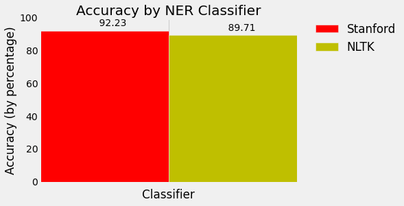
nltk_accuracy = accuracy(reference_annotations, nltk_formatted_prediction)
print(nltk_accuracy)
```
哇,準確率為`.8971`!
現在讓我們測試斯坦福分類器。 由于此分類器以元組形式生成輸出,因此測試不需要更多的數據操作。
```py
st = StanfordNERTagger('/usr/share/stanford-ner/classifiers/english.all.3class.distsim.crf.ser.gz',
'/usr/share/stanford-ner/stanford-ner.jar',
encoding='utf-8')
stanford_prediction = st.tag(pure_tokens)
stanford_accuracy = accuracy(reference_annotations, stanford_prediction)
print(stanford_accuracy)
```
`.9223`的準確率!更好!
如果你想繪制這個,這里有一些額外的代碼。 如果你想深入了解這如何工作,查看 matplotlib 系列:
```py
import numpy as np
import matplotlib.pyplot as plt
from matplotlib import style
style.use('fivethirtyeight')
N = 1
ind = np.arange(N) # the x locations for the groups
width = 0.35 # the width of the bars
fig, ax = plt.subplots()
stanford_percentage = stanford_accuracy * 100
rects1 = ax.bar(ind, stanford_percentage, width, color='r')
nltk_percentage = nltk_accuracy * 100
rects2 = ax.bar(ind+width, nltk_percentage, width, color='y')
# add some text for labels, title and axes ticks
ax.set_xlabel('Classifier')
ax.set_ylabel('Accuracy (by percentage)')
ax.set_title('Accuracy by NER Classifier')
ax.set_xticks(ind+width)
ax.set_xticklabels( ('') )
ax.legend( (rects1[0], rects2[0]), ('Stanford', 'NLTK'), bbox_to_anchor=(1.05, 1), loc=2, borderaxespad=0. )
def autolabel(rects):
# attach some text labels
for rect in rects:
height = rect.get_height()
ax.text(rect.get_x()+rect.get_width()/2., 1.02*height, '%10.2f' % float(height),
ha='center', va='bottom')
autolabel(rects1)
autolabel(rects2)
plt.show()
```
## 二十四、測試 NLTK 和斯坦福 NER 標記器的速度
> [Chuck Dishmon](http://chuckdishmon.github.io/) 的客座文章。
我們已經測試了我們的 NER 分類器的準確性,但是在決定使用哪個分類器時,還有更多的問題需要考慮。 接下來我們來測試速度吧!
我們知道我們正在比較同一個東西,我們將在同一篇文章中進行測試。 使用 NBC 新聞里的這個片段吧:
```
House Speaker John Boehner became animated Tuesday over the proposed Keystone Pipeline, castigating the Obama administration for not having approved the project yet.
Republican House Speaker John Boehner says there's "nothing complex about the Keystone Pipeline," and that it's time to build it.
"Complex? You think the Keystone Pipeline is complex?!" Boehner responded to a questioner. "It's been under study for five years! We build pipelines in America every day. Do you realize there are 200,000 miles of pipelines in the United States?"
The speaker went on: "And the only reason the president's involved in the Keystone Pipeline is because it crosses an international boundary. Listen, we can build it. There's nothing complex about the Keystone Pipeline -- it's time to build it."
Boehner said the president had no excuse at this point to not give the pipeline the go-ahead after the State Department released a report on Friday indicating the project would have a minimal impact on the environment.
Republicans have long pushed for construction of the project, which enjoys some measure of Democratic support as well. The GOP is considering conditioning an extension of the debt limit on approval of the project by Obama.
The White House, though, has said that it has no timetable for a final decision on the project.
```
首先,我們執行導入,通過閱讀和分詞來處理文章。
```py
# -*- coding: utf-8 -*-
import nltk
import os
import numpy as np
import matplotlib.pyplot as plt
from matplotlib import style
from nltk import pos_tag
from nltk.tag import StanfordNERTagger
from nltk.tokenize import word_tokenize
style.use('fivethirtyeight')
# Process text
def process_text(txt_file):
raw_text = open("/usr/share/news_article.txt").read()
token_text = word_tokenize(raw_text)
return token_text
```
很棒! 現在讓我們寫一些函數來拆分我們的分類任務。 因為 NLTK NEG 分類器需要 POS 標簽,所以我們會在我們的 NLTK 函數中加入 POS 標簽。
```py
# Stanford NER tagger
def stanford_tagger(token_text):
st = StanfordNERTagger('/usr/share/stanford-ner/classifiers/english.all.3class.distsim.crf.ser.gz',
'/usr/share/stanford-ner/stanford-ner.jar',
encoding='utf-8')
ne_tagged = st.tag(token_text)
return(ne_tagged)
# NLTK POS and NER taggers
def nltk_tagger(token_text):
tagged_words = nltk.pos_tag(token_text)
ne_tagged = nltk.ne_chunk(tagged_words)
return(ne_tagged)
```
每個分類器都需要讀取文章,并對命名實體進行分類,所以我們將這些函數包裝在一個更大的函數中,使計時變得簡單。
```py
def stanford_main():
print(stanford_tagger(process_text(txt_file)))
def nltk_main():
print(nltk_tagger(process_text(txt_file)))
```
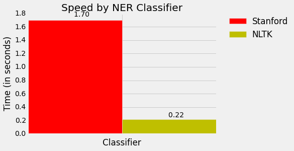
當我們調用我們的程序時,我們調用這些函數。 我們將在`os.times()`函數調用中包裝我們的`stanford_main()`和`nltk_main()`函數,取第四個索引,它是經過的時間。 然后我們將圖繪制我們的結果。
```py
if __name__ == '__main__':
stanford_t0 = os.times()[4]
stanford_main()
stanford_t1 = os.times()[4]
stanford_total_time = stanford_t1 - stanford_t0
nltk_t0 = os.times()[4]
nltk_main()
nltk_t1 = os.times()[4]
nltk_total_time = nltk_t1 - nltk_t0
time_plot(stanford_total_time, nltk_total_time)
```
對于我們的繪圖,我們使用`time_plot()`函數:
```py
def time_plot(stanford_total_time, nltk_total_time):
N = 1
ind = np.arange(N) # the x locations for the groups
width = 0.35 # the width of the bars
stanford_total_time = stanford_total_time
nltk_total_time = nltk_total_time
fig, ax = plt.subplots()
rects1 = ax.bar(ind, stanford_total_time, width, color='r')
rects2 = ax.bar(ind+width, nltk_total_time, width, color='y')
# Add text for labels, title and axes ticks
ax.set_xlabel('Classifier')
ax.set_ylabel('Time (in seconds)')
ax.set_title('Speed by NER Classifier')
ax.set_xticks(ind+width)
ax.set_xticklabels( ('') )
ax.legend( (rects1[0], rects2[0]), ('Stanford', 'NLTK'), bbox_to_anchor=(1.05, 1), loc=2, borderaxespad=0. )
def autolabel(rects):
# attach some text labels
for rect in rects:
height = rect.get_height()
ax.text(rect.get_x()+rect.get_width()/2., 1.02*height, '%10.2f' % float(height),
ha='center', va='bottom')
autolabel(rects1)
autolabel(rects2)
plt.show()
```
哇,NLTK 像閃電一樣快! 看來斯坦福更準確,但 NLTK 更快。 當平衡我們偏愛的精確度,和所需的計算資源時,這是需要知道的重要信息。
但是等等,還是有問題。我們的輸出比較丑陋! 這是斯坦福大學的一個小樣本:
```py
[('House', 'ORGANIZATION'), ('Speaker', 'O'), ('John', 'PERSON'), ('Boehner', 'PERSON'), ('became', 'O'), ('animated', 'O'), ('Tuesday', 'O'), ('over', 'O'), ('the', 'O'), ('proposed', 'O'), ('Keystone', 'ORGANIZATION'), ('Pipeline', 'ORGANIZATION'), (',', 'O'), ('castigating', 'O'), ('the', 'O'), ('Obama', 'PERSON'), ('administration', 'O'), ('for', 'O'), ('not', 'O'), ('having', 'O'), ('approved', 'O'), ('the', 'O'), ('project', 'O'), ('yet', 'O'), ('.', 'O')
```
以及 NLTK:
```
(S
(ORGANIZATION House/NNP)
Speaker/NNP
(PERSON John/NNP Boehner/NNP)
became/VBD
animated/VBN
Tuesday/NNP
over/IN
the/DT
proposed/VBN
(PERSON Keystone/NNP Pipeline/NNP)
,/,
castigating/VBG
the/DT
(ORGANIZATION Obama/NNP)
administration/NN
for/IN
not/RB
having/VBG
approved/VBN
the/DT
project/NN
yet/RB
./.
```
讓我們在下個教程中,將它們轉為可讀的形式。
## 使用 BIO 標簽創建可讀的命名實體列表
> [Chuck Dishmon](http://chuckdishmon.github.io/) 的客座文章。
現在我們已經完成了測試,讓我們將我們的命名實體轉為良好的可讀格式。
再次,我們將使用來自 NBC 新聞的同一篇新聞:
```
House Speaker John Boehner became animated Tuesday over the proposed Keystone Pipeline, castigating the Obama administration for not having approved the project yet.
Republican House Speaker John Boehner says there's "nothing complex about the Keystone Pipeline," and that it's time to build it.
"Complex? You think the Keystone Pipeline is complex?!" Boehner responded to a questioner. "It's been under study for five years! We build pipelines in America every day. Do you realize there are 200,000 miles of pipelines in the United States?"
The speaker went on: "And the only reason the president's involved in the Keystone Pipeline is because it crosses an international boundary. Listen, we can build it. There's nothing complex about the Keystone Pipeline -- it's time to build it."
Boehner said the president had no excuse at this point to not give the pipeline the go-ahead after the State Department released a report on Friday indicating the project would have a minimal impact on the environment.
Republicans have long pushed for construction of the project, which enjoys some measure of Democratic support as well. The GOP is considering conditioning an extension of the debt limit on approval of the project by Obama.
The White House, though, has said that it has no timetable for a final decision on the project.
```
我們的 NTLK 輸出已經是樹了(只需要最后一步),所以讓我們來看看我們的斯坦福輸出。 我們將對標記進行 BIO 標記,B 分配給命名實體的開始,I 分配給內部,O 分配給其他。 例如,如果我們的句子是`Barack Obama went to Greece today`,我們應該把它標記為`Barack-B Obama-I went-O to-O Greece-B today-O`。 為此,我們將編寫一系列條件來檢查當前和以前的標記的`O`標簽。
```py
# -*- coding: utf-8 -*-
import nltk
import os
import numpy as np
import matplotlib.pyplot as plt
from matplotlib import style
from nltk import pos_tag
from nltk.tag import StanfordNERTagger
from nltk.tokenize import word_tokenize
from nltk.chunk import conlltags2tree
from nltk.tree import Tree
style.use('fivethirtyeight')
# Process text
def process_text(txt_file):
raw_text = open("/usr/share/news_article.txt").read()
token_text = word_tokenize(raw_text)
return token_text
# Stanford NER tagger
def stanford_tagger(token_text):
st = StanfordNERTagger('/usr/share/stanford-ner/classifiers/english.all.3class.distsim.crf.ser.gz',
'/usr/share/stanford-ner/stanford-ner.jar',
encoding='utf-8')
ne_tagged = st.tag(token_text)
return(ne_tagged)
# NLTK POS and NER taggers
def nltk_tagger(token_text):
tagged_words = nltk.pos_tag(token_text)
ne_tagged = nltk.ne_chunk(tagged_words)
return(ne_tagged)
# Tag tokens with standard NLP BIO tags
def bio_tagger(ne_tagged):
bio_tagged = []
prev_tag = "O"
for token, tag in ne_tagged:
if tag == "O": #O
bio_tagged.append((token, tag))
prev_tag = tag
continue
if tag != "O" and prev_tag == "O": # Begin NE
bio_tagged.append((token, "B-"+tag))
prev_tag = tag
elif prev_tag != "O" and prev_tag == tag: # Inside NE
bio_tagged.append((token, "I-"+tag))
prev_tag = tag
elif prev_tag != "O" and prev_tag != tag: # Adjacent NE
bio_tagged.append((token, "B-"+tag))
prev_tag = tag
return bio_tagged
```
現在我們將 BIO 標記后的標記寫入樹中,因此它們與 NLTK 輸出格式相同。
```py
# Create tree
def stanford_tree(bio_tagged):
tokens, ne_tags = zip(*bio_tagged)
pos_tags = [pos for token, pos in pos_tag(tokens)]
conlltags = [(token, pos, ne) for token, pos, ne in zip(tokens, pos_tags, ne_tags)]
ne_tree = conlltags2tree(conlltags)
return ne_tree
```
遍歷并解析出所有命名實體:
```py
# Parse named entities from tree
def structure_ne(ne_tree):
ne = []
for subtree in ne_tree:
if type(subtree) == Tree: # If subtree is a noun chunk, i.e. NE != "O"
ne_label = subtree.label()
ne_string = " ".join([token for token, pos in subtree.leaves()])
ne.append((ne_string, ne_label))
return ne
```
在我們的調用中,我們把所有附加函數聚到一起。
```py
def stanford_main():
print(structure_ne(stanford_tree(bio_tagger(stanford_tagger(process_text(txt_file))))))
def nltk_main():
print(structure_ne(nltk_tagger(process_text(txt_file))))
```
之后調用這些函數:
```py
if __name__ == '__main__':
stanford_main()
nltk_main()
```
這里是來自斯坦福的看起來不錯的輸出:
```py
[('House', 'ORGANIZATION'), ('John Boehner', 'PERSON'), ('Keystone Pipeline', 'ORGANIZATION'), ('Obama', 'PERSON'), ('Republican House', 'ORGANIZATION'), ('John Boehner', 'PERSON'), ('Keystone Pipeline', 'ORGANIZATION'), ('Keystone Pipeline', 'ORGANIZATION'), ('Boehner', 'PERSON'), ('America', 'LOCATION'), ('United States', 'LOCATION'), ('Keystone Pipeline', 'ORGANIZATION'), ('Keystone Pipeline', 'ORGANIZATION'), ('Boehner', 'PERSON'), ('State Department', 'ORGANIZATION'), ('Republicans', 'MISC'), ('Democratic', 'MISC'), ('GOP', 'MISC'), ('Obama', 'PERSON'), ('White House', 'LOCATION')]
```
以及來自 NLTK 的:
```py
[('House', 'ORGANIZATION'), ('John Boehner', 'PERSON'), ('Keystone Pipeline', 'PERSON'), ('Obama', 'ORGANIZATION'), ('Republican', 'ORGANIZATION'), ('House', 'ORGANIZATION'), ('John Boehner', 'PERSON'), ('Keystone Pipeline', 'ORGANIZATION'), ('Keystone Pipeline', 'ORGANIZATION'), ('Boehner', 'PERSON'), ('America', 'GPE'), ('United States', 'GPE'), ('Keystone Pipeline', 'ORGANIZATION'), ('Listen', 'PERSON'), ('Keystone', 'ORGANIZATION'), ('Boehner', 'PERSON'), ('State Department', 'ORGANIZATION'), ('Democratic', 'ORGANIZATION'), ('GOP', 'ORGANIZATION'), ('Obama', 'PERSON'), ('White House', 'FACILITY')]
```
分塊在一起,可讀性強。不錯!
