1.3 NumPy：創建和操作數值數據 · SciPy Lecture Notes 中文版

# 1.3 NumPy：創建和操作數值數據 > 作者：Emmanuelle Gouillart、Didrik Pinte、Ga?l Varoquaux 和 Pauli Virtanen 本章給出關于Numpy概述，Numpy是Python中高效數值計算的核心工具。 ## 1.3.1 Numpy 數組對象 ### 1.3.1.1 什么是Numpy以及Numpy數組？ #### 1.3.1.1.1 Numpy數組 **Python對象：** * 高級數值對象：整數、浮點 * 容器：列表（無成本插入和附加），字典（快速查找） **Numpy提供：** * 對于多維度數組的Python擴展包 * 更貼近硬件（高效） * 為科學計算設計（方便） * 也稱為_面向數組計算_ In?[1]: ``` import numpy as np a = np.array([0, 1, 2, 3]) a ``` Out[1]: ``` array([0, 1, 2, 3]) ``` 例如，數組包含： * 實驗或模擬在離散時間階段的值 * 測量設備記錄的信號，比如聲波 * 圖像的像素、灰度或顏色 * 用不同X-Y-Z位置測量的3-D數據，例如MRI掃描 ... **為什么有用：**提供了高速數值操作的節省內存的容器。 In?[2]: ``` L = range(1000) %timeit [i**2 for i in L] ``` ``` 10000 loops, best of 3: 93.7 μs per loop ``` In?[4]: ``` a = np.arange(1000) %timeit a**2 ``` ``` 100000 loops, best of 3: 2.16 μs per loop ``` #### 1.3.1.1.2 Numpy參考文檔 * 線上: [http://docs.scipy.org/](http://docs.scipy.org/) * 交互幫助: ``` np.array? String Form:<built-in function array> Docstring: array(object, dtype=None, copy=True, order=None, subok=False, ndmin=0, ... ``` 查找東西： In?[6]: ``` np.lookfor('create array') ``` ``` Search results for 'create array' --------------------------------- numpy.array Create an array. numpy.memmap Create a memory-map to an array stored in a *binary* file on disk. numpy.diagflat Create a two-dimensional array with the flattened input as a diagonal. numpy.fromiter Create a new 1-dimensional array from an iterable object. numpy.partition Return a partitioned copy of an array. numpy.ma.diagflat Create a two-dimensional array with the flattened input as a diagonal. numpy.ctypeslib.as_array Create a numpy array from a ctypes array or a ctypes POINTER. numpy.ma.make_mask Create a boolean mask from an array. numpy.ctypeslib.as_ctypes Create and return a ctypes object from a numpy array. Actually numpy.ma.mrecords.fromarrays Creates a mrecarray from a (flat) list of masked arrays. numpy.lib.format.open_memmap Open a .npy file as a memory-mapped array. numpy.ma.MaskedArray.__new__ Create a new masked array from scratch. numpy.lib.arrayterator.Arrayterator Buffered iterator for big arrays. numpy.ma.mrecords.fromtextfile Creates a mrecarray from data stored in the file `filename`. numpy.asarray Convert the input to an array. numpy.ndarray ndarray(shape, dtype=float, buffer=None, offset=0, numpy.recarray Construct an ndarray that allows field access using attributes. numpy.chararray chararray(shape, itemsize=1, unicode=False, buffer=None, offset=0, numpy.pad Pads an array. numpy.sum Sum of array elements over a given axis. numpy.asanyarray Convert the input to an ndarray, but pass ndarray subclasses through. numpy.copy Return an array copy of the given object. numpy.diag Extract a diagonal or construct a diagonal array. numpy.load Load arrays or pickled objects from ``.npy``, ``.npz`` or pickled files. numpy.sort Return a sorted copy of an array. numpy.array_equiv Returns True if input arrays are shape consistent and all elements equal. numpy.dtype Create a data type object. numpy.choose Construct an array from an index array and a set of arrays to choose from. numpy.nditer Efficient multi-dimensional iterator object to iterate over arrays. numpy.swapaxes Interchange two axes of an array. numpy.full_like Return a full array with the same shape and type as a given array. numpy.ones_like Return an array of ones with the same shape and type as a given array. numpy.empty_like Return a new array with the same shape and type as a given array. numpy.zeros_like Return an array of zeros with the same shape and type as a given array. numpy.asarray_chkfinite Convert the input to an array, checking for NaNs or Infs. numpy.diag_indices Return the indices to access the main diagonal of an array. numpy.ma.choose Use an index array to construct a new array from a set of choices. numpy.chararray.tolist a.tolist() numpy.matlib.rand Return a matrix of random values with given shape. numpy.savez_compressed Save several arrays into a single file in compressed ``.npz`` format. numpy.ma.empty_like Return a new array with the same shape and type as a given array. numpy.ma.make_mask_none Return a boolean mask of the given shape, filled with False. numpy.ma.mrecords.fromrecords Creates a MaskedRecords from a list of records. numpy.around Evenly round to the given number of decimals. numpy.source Print or write to a file the source code for a Numpy object. numpy.diagonal Return specified diagonals. numpy.histogram2d Compute the bi-dimensional histogram of two data samples. numpy.fft.ifft Compute the one-dimensional inverse discrete Fourier Transform. numpy.fft.ifftn Compute the N-dimensional inverse discrete Fourier Transform. numpy.busdaycalendar A business day calendar object that efficiently stores information ``` ``` np.con*? np.concatenate np.conj np.conjugate np.convolve ``` #### 1.3.1.1.3 導入慣例導入numpy的推薦慣例是： In?[8]: ``` import numpy as np ``` ### 1.3.1.2 創建數組 #### 1.3.1.2.1 手動構建數組 * 1-D： In?[9]: ``` a = np.array([0, 1, 2, 3]) a ``` Out[9]: ``` array([0, 1, 2, 3]) ``` In?[10]: ``` a.ndim ``` Out[10]: ``` 1 ``` In?[11]: ``` a.shape ``` Out[11]: ``` (4,) ``` In?[12]: ``` len(a) ``` Out[12]: ``` 4 ``` * 2-D，3-D，...： In?[13]: ``` b = np.array([[0, 1, 2], [3, 4, 5]]) # 2 x 3 數組 b ``` Out[13]: ``` array([[0, 1, 2], [3, 4, 5]]) ``` In?[14]: ``` b.ndim ``` Out[14]: ``` 2 ``` In?[15]: ``` b.shape ``` Out[15]: ``` (2, 3) ``` In?[16]: ``` len(b) # 返回一個緯度的大小 ``` Out[16]: ``` 2 ``` In?[17]: ``` c = np.array([[[1], [2]], [[3], [4]]]) c ``` Out[17]: ``` array([[[1], [2]], [[3], [4]]]) ``` In?[18]: ``` c.shape ``` Out[18]: ``` (2, 2, 1) ``` **練習：簡單數組** * 創建一個簡單的二維數組。首先，重復上面的例子。然后接著你自己的：在第一行從后向前數奇數，接著第二行數偶數？ * 在這些數組上使用函數[len()](http://docs.python.org/2.7/library/functions.html#len)、numpy.shape()。他們有什么關系？與數組的`ndim`屬性間呢？ #### 1.3.1.2.2 創建數組的函數實際上，我們很少一個項目接一個項目輸入... * 均勻分布： In?[19]: ``` a = np.arange(10) # 0 .. n-1 (!) a ``` Out[19]: ``` array([0, 1, 2, 3, 4, 5, 6, 7, 8, 9]) ``` In?[20]: ``` b = np.arange(1, 9, 2) # 開始，結束（不包含），步長 b ``` Out[20]: ``` array([1, 3, 5, 7]) ``` * 或者通過一些數據點： In?[1]: ``` c = np.linspace(0, 1, 6) # 起點、終點、數據點 c ``` Out[1]: ``` array([ 0\. , 0.2, 0.4, 0.6, 0.8, 1\. ]) ``` In?[2]: ``` d = np.linspace(0, 1, 5, endpoint=False) d ``` Out[2]: ``` array([ 0\. , 0.2, 0.4, 0.6, 0.8]) ``` * 普通數組： In?[3]: ``` a = np.ones((3, 3)) # 提示: (3, 3) 是元組 a ``` Out[3]: ``` array([[ 1., 1., 1.], [ 1., 1., 1.], [ 1., 1., 1.]]) ``` In?[4]: ``` b = np.zeros((2, 2)) b ``` Out[4]: ``` array([[ 0., 0.], [ 0., 0.]]) ``` In?[5]: ``` c = np.eye(3) c ``` Out[5]: ``` array([[ 1., 0., 0.], [ 0., 1., 0.], [ 0., 0., 1.]]) ``` In?[6]: ``` d = np.diag(np.array([1, 2, 3, 4])) d ``` Out[6]: ``` array([[1, 0, 0, 0], [0, 2, 0, 0], [0, 0, 3, 0], [0, 0, 0, 4]]) ``` * `np.random`: 隨機數 (Mersenne Twister PRNG) : In?[7]: ``` a = np.random.rand(4) # [0, 1] 的均勻分布 a ``` Out[7]: ``` array([ 0.05504731, 0.38154156, 0.39639478, 0.22379146]) ``` In?[8]: ``` b = np.random.randn(4) # 高斯 b ``` Out[8]: ``` array([ 0.9895903 , 1.85061188, 1.0021666 , -0.63782069]) ``` In?[9]: ``` np.random.seed(1234) # 設置隨機種子 ``` In?[10]: ``` np.random.rand? ``` **練習：用函數創建數組** * 實驗用`arange`、`linspace`、`ones`、`zeros`、`eye`和`diag`。 * 用隨機數創建不同類型的數組。 * 在創建帶有隨機數的數組前設定種子。 * 看一下函數`np.empty`。它能做什么？什么時候會比較有用？ ### 1.3.1.3基礎數據類型你可能已經發現，在一些情況下，數組元素顯示帶有點（即 2\. VS 2）。這是因為所使用的數據類型不同： In?[12]: ``` a = np.array([1, 2, 3]) a.dtype ``` Out[12]: ``` dtype('int64') ``` In?[13]: ``` b = np.array([1., 2., 3.]) b ``` Out[13]: ``` array([ 1., 2., 3.]) ``` 不同的數據類型可以更緊湊的在內存中存儲數據，但是大多數時候我們都只是操作浮點數據。注意，在上面的例子中，Numpy自動從輸入中識別了數據類型。你可以明確的指定想要的類型： In?[1]: ``` c = np.array([1, 2, 3], dtype=float) c.dtype ``` Out[1]: ``` dtype('float64') ``` **默認**數據類型是浮點: In?[2]: ``` a = np.ones((3, 3)) a.dtype ``` Out[2]: ``` dtype('float64') ``` 其他類型： **復數**： In?[4]: ``` d = np.array([1+2j, 3+4j, 5+6*1j]) d.dtype ``` Out[4]: ``` dtype('complex128') ``` **布爾**： In?[5]: ``` e = np.array([True, False, False, True]) e.dtype ``` Out[5]: ``` dtype('bool') ``` **字符**： In?[6]: ``` f = np.array(['Bonjour', 'Hello', 'Hallo',]) f.dtype # <--- 包含最多7個字母的字符 ``` Out[6]: ``` dtype('S7') ``` **更多**： * int32 * int64 * unit32 * unit64 ### 1.3.1.4基本可視化現在我們有了第一個數組，我們將要進行可視化。從_pylab_模式啟動IPython。 ``` ipython --pylab ``` 或notebook： ``` ipython notebook --pylab=inline ``` 或者如果IPython已經啟動，那么： In?[119]: ``` %pylab ``` ``` Using matplotlib backend: MacOSX Populating the interactive namespace from numpy and matplotlib ``` 或者從Notebook中： In?[121]: ``` %pylab inline ``` ``` Populating the interactive namespace from numpy and matplotlib ``` `inline` 對notebook來說很重要，以便繪制的圖片在notebook中顯示而不是在新窗口顯示。 _Matplotlib_是2D制圖包。我們可以像下面這樣導入它的方法： In?[10]: ``` import matplotlib.pyplot as plt #整潔形式 ``` 然后使用（注你需要顯式的使用 `show` ）: ``` plt.plot(x, y) # 線圖 plt.show() # <-- 顯示圖表（使用pylab的話不需要） ``` 或者，如果你使用 `pylab`： ``` plt.plot(x, y) # 線圖 ``` 在腳本中推薦使用 `import matplotlib.pyplot as plt`。而交互的探索性工作中用 `pylab`。 * 1D作圖： In?[12]: ``` x = np.linspace(0, 3, 20) y = np.linspace(0, 9, 20) plt.plot(x, y) # 線圖 ``` Out[12]: ``` [<matplotlib.lines.Line2D at 0x1068f38d0>] ``` ![](https://box.kancloud.cn/2016-03-21_56efdc06c6133.png) In?[13]: ``` plt.plot(x, y, 'o') # 點圖 ``` Out[13]: ``` [<matplotlib.lines.Line2D at 0x106b32090>] ``` ![](https://box.kancloud.cn/2016-03-21_56efdc06d87e5.png) * 2D 作圖: In?[14]: ``` image = np.random.rand(30, 30) plt.imshow(image, cmap=plt.cm.hot) plt.colorbar() ``` Out[14]: ``` <matplotlib.colorbar.Colorbar instance at 0x106a095f0> ``` ![](https://box.kancloud.cn/2016-03-21_56efdc06e9180.png) 更多請見matplotlib部分（暫缺） **練習**：簡單可視化畫出簡單的數組：cosine作為時間的一個函數以及2D矩陣。在2D矩陣上試試使用 `gray` colormap。 #### 1.3.1.5索引和切片數組的項目可以用與其他Python序列（比如：列表）一樣的方式訪問和賦值： In?[15]: ``` a = np.arange(10) a ``` Out[15]: ``` array([0, 1, 2, 3, 4, 5, 6, 7, 8, 9]) ``` In?[16]: ``` a[0], a[2], a[-1] ``` Out[16]: ``` (0, 2, 9) ``` **警告**：索引從0開始與其他的Python序列（以及C/C++）一樣。相反，在Fortran或者Matlab索引從1開始。使用常用的Python風格來反轉一個序列也是支持的： In?[17]: ``` a[::-1] ``` Out[17]: ``` array([9, 8, 7, 6, 5, 4, 3, 2, 1, 0]) ``` 對于多維數組，索引是整數的元組： In?[18]: ``` a = np.diag(np.arange(3)) a ``` Out[18]: ``` array([[0, 0, 0], [0, 1, 0], [0, 0, 2]]) ``` In?[19]: ``` a[1, 1] ``` Out[19]: ``` 1 ``` In?[21]: ``` a[2, 1] = 10 # 第三行，第二列 a ``` Out[21]: ``` array([[ 0, 0, 0], [ 0, 1, 0], [ 0, 10, 2]]) ``` In?[22]: ``` a[1] ``` Out[22]: ``` array([0, 1, 0]) ``` **注**： * 在2D數組中，第一個緯度對應行，第二個緯度對應列。 * 對于多維度數組 `a`，a[0]被解釋為提取在指定緯度的所有元素 **切片**：數組與其他Python序列也可以被切片： In?[23]: ``` a = np.arange(10) a ``` Out[23]: ``` array([0, 1, 2, 3, 4, 5, 6, 7, 8, 9]) ``` In?[24]: ``` a[2:9:3] # [開始:結束:步長] ``` Out[24]: ``` array([2, 5, 8]) ``` 注意最后一個索引是不包含的！： In?[25]: ``` a[:4] ``` Out[25]: ``` array([0, 1, 2, 3]) ``` 切片的三個元素都不是必選：默認情況下，起點是0，結束是最后一個，步長是1： In?[26]: ``` a[1:3] ``` Out[26]: ``` array([1, 2]) ``` In?[27]: ``` a[::2] ``` Out[27]: ``` array([0, 2, 4, 6, 8]) ``` In?[28]: ``` a[3:] ``` Out[28]: ``` array([3, 4, 5, 6, 7, 8, 9]) ``` Numpy索引和切片的一個小說明... ![numpy_indexing](http://scipy-lectures.github.io/_images/numpy_indexing.png) 賦值和切片可以結合在一起： In?[29]: ``` a = np.arange(10) a[5:] = 10 a ``` Out[29]: ``` array([ 0, 1, 2, 3, 4, 10, 10, 10, 10, 10]) ``` In?[30]: ``` b = np.arange(5) a[5:] = b[::-1] a ``` Out[30]: ``` array([0, 1, 2, 3, 4, 4, 3, 2, 1, 0]) ``` **練習：索引與切片** * 試試切片的特色，用起點、結束和步長：從linspace開始，試著從后往前獲得奇數，從前往后獲得偶數。重現上面示例中的切片。你需要使用下列表達式創建這個數組： In?[31]: ``` np.arange(6) + np.arange(0, 51, 10)[:, np.newaxis] ``` Out[31]: ``` array([[ 0, 1, 2, 3, 4, 5], [10, 11, 12, 13, 14, 15], [20, 21, 22, 23, 24, 25], [30, 31, 32, 33, 34, 35], [40, 41, 42, 43, 44, 45], [50, 51, 52, 53, 54, 55]]) ``` **練習：數組創建** 創建下列的數組（用正確的數據類型）： ``` [[1, 1, 1, 1], [1, 1, 1, 1], [1, 1, 1, 2], [1, 6, 1, 1]] [[0., 0., 0., 0., 0.], [2., 0., 0., 0., 0.], [0., 3., 0., 0., 0.], [0., 0., 4., 0., 0.], [0., 0., 0., 5., 0.], [0., 0., 0., 0., 6.]] ``` 參考標準：每個數組提示：每個數組元素可以像列表一樣訪問，即a[1] 或 a[1, 2]。提示：看一下 `diag` 的文檔字符串。 **練習：創建平鋪數組** 看一下 `np.tile` 的文檔，是用這個函數創建這個數組： ``` [[4, 3, 4, 3, 4, 3], [2, 1, 2, 1, 2, 1], [4, 3, 4, 3, 4, 3], [2, 1, 2, 1, 2, 1]] ``` ### 1.3.1.6 副本和視圖切片操作創建原數組的一個**視圖**，這只是訪問數組數據一種方式。因此，原始的數組并不是在內存中復制。你可以用 `np.may_share_memory()` 來確認兩個數組是否共享相同的內存塊。但是請注意，這種方式使用啟發式，可能產生漏報。 **當修改視圖時，原始數據也被修改： In?[32]: ``` a = np.arange(10) a ``` Out[32]: ``` array([0, 1, 2, 3, 4, 5, 6, 7, 8, 9]) ``` In?[33]: ``` b = a[::2] b ``` Out[33]: ``` array([0, 2, 4, 6, 8]) ``` In?[34]: ``` np.may_share_memory(a, b) ``` Out[34]: ``` True ``` In?[36]: ``` b[0] = 12 b ``` Out[36]: ``` array([12, 2, 4, 6, 8]) ``` In?[37]: ``` a # (!) ``` Out[37]: ``` array([12, 1, 2, 3, 4, 5, 6, 7, 8, 9]) ``` In?[38]: ``` a = np.arange(10) c = a[::2].copy() # 強制復制 c[0] = 12 a ``` Out[38]: ``` array([0, 1, 2, 3, 4, 5, 6, 7, 8, 9]) ``` In?[39]: ``` np.may_share_memory(a, c) ``` Out[39]: ``` False ``` 乍看之下這種行為可能有些奇怪，但是這樣做節省了內存和時間。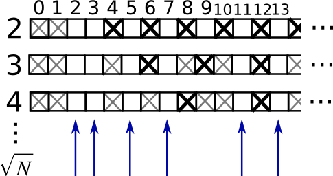 **實例：素數篩選** ![prime](http://scipy-lectures.github.io/_images/prime-sieve.png) 用篩選法計算0-99之間的素數 * 構建一個名為 `_prime` 形狀是 (100,) 的布爾數組，在初始將值都設為True： In?[40]: ``` is_prime = np.ones((100,), dtype=bool) ``` * 將不屬于素數的0，1去掉 In?[41]: ``` is_prime[:2] = 0 ``` 對于從2開始的整數 `j` ，化掉它的倍數： In?[42]: ``` N_max = int(np.sqrt(len(is_prime))) for j in range(2, N_max): is_prime[2*j::j] = False ``` * 看一眼 `help(np.nonzero)`，然后打印素數 * 接下來: * 將上面的代碼放入名為 `prime_sieve.py` 的腳本文件 * 運行檢查一下時候有效 * 使用[埃拉托斯特尼篩法](http://en.wikipedia.org/wiki/Sieve_of_Eratosthenes)的優化建議 1. 跳過已知不是素數的 `j` 2. 第一個應該被劃掉的數是$j^2$ #### 1.3.1.7象征索引 Numpy數組可以用切片索引，也可以用布爾或整形數組（面具）。這個方法也被稱為象征索引。它創建一個副本而不是視圖。 #### 1.3.1.7.1使用布爾面具 In?[44]: ``` np.random.seed(3) a = np.random.random_integers(0, 20, 15) a ``` Out[44]: ``` array([10, 3, 8, 0, 19, 10, 11, 9, 10, 6, 0, 20, 12, 7, 14]) ``` In?[45]: ``` (a % 3 == 0) ``` Out[45]: ``` array([False, True, False, True, False, False, False, True, False, True, True, False, True, False, False], dtype=bool) ``` In?[47]: ``` mask = (a % 3 == 0) extract_from_a = a[mask] # 或, a[a%3==0] extract_from_a # 用面具抽取一個子數組 ``` Out[47]: ``` array([ 3, 0, 9, 6, 0, 12]) ``` 賦值給子數組時，用面具索引非常有用： In?[48]: ``` a[a % 3 == 0] = -1 a ``` Out[48]: ``` array([10, -1, 8, -1, 19, 10, 11, -1, 10, -1, -1, 20, -1, 7, 14]) ``` #### 1.3.1.7.2 用整型數組索引 In?[49]: ``` a = np.arange(0, 100, 10) a ``` Out[49]: ``` array([ 0, 10, 20, 30, 40, 50, 60, 70, 80, 90]) ``` 索引可以用整型數組完成，其中相同的索引重復了幾次： In?[50]: ``` a[[2, 3, 2, 4, 2]] # 注：[2, 3, 2, 4, 2] 是Python列表 ``` Out[50]: ``` array([20, 30, 20, 40, 20]) ``` 用這種類型的索引可以分配新值： In?[51]: ``` a[[9, 7]] = -100 a ``` Out[51]: ``` array([ 0, 10, 20, 30, 40, 50, 60, -100, 80, -100]) ``` 當一個新數組用整型數組索引創建時，新數組有相同的形狀，而不是整數數組： In?[52]: ``` a = np.arange(10) idx = np.array([[3, 4], [9, 7]]) idx.shape ``` Out[52]: ``` (2, 2) ``` In?[53]: ``` a[idx] ``` Out[53]: ``` array([[3, 4], [9, 7]]) ``` 下圖展示了多種象征索引的應用 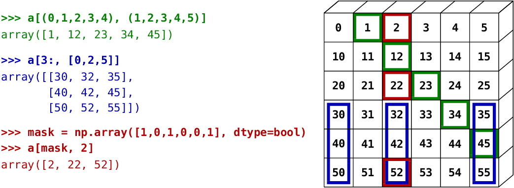![numpy_fancy_indexing](http://scipy-lectures.github.io/_images/numpy_fancy_indexing.png) **練習：象征索引** * 同樣，重新生成上圖中所示的象征索引 * 用左側的象征索引和右側的數組創建在為一個數組賦值，例如，設置上圖數組的一部分為0。 ## 1.3.2 數組的數值操作 ### 1.3.2.1 元素級操作 #### 1.3.2.1.1 基礎操作標量: In?[54]: ``` a = np.array([1, 2, 3, 4]) a + 1 ``` Out[54]: ``` array([2, 3, 4, 5]) ``` In?[55]: ``` 2**a ``` Out[55]: ``` array([ 2, 4, 8, 16]) ``` 所有運算是在元素級別上操作： In?[56]: ``` b = np.ones(4) + 1 a - b ``` Out[56]: ``` array([-1., 0., 1., 2.]) ``` In?[57]: ``` a * b ``` Out[57]: ``` array([ 2., 4., 6., 8.]) ``` In?[58]: ``` j = np.arange(5) 2**(j + 1) - j ``` Out[58]: ``` array([ 2, 3, 6, 13, 28]) ``` 這些操作當然也比你用純Python實現好快得多： In?[60]: ``` a = np.arange(10000) %timeit a + 1 ``` ``` 100000 loops, best of 3: 11 μs per loop ``` In?[61]: ``` l = range(10000) %timeit [i+1 for i in l] ``` ``` 1000 loops, best of 3: 560 μs per loop ``` **注意：數組相乘不是矩陣相乘：** In?[62]: ``` c = np.ones((3, 3)) c * c # 不是矩陣相乘！ ``` Out[62]: ``` array([[ 1., 1., 1.], [ 1., 1., 1.], [ 1., 1., 1.]]) ``` **注：矩陣相乘：** In?[63]: ``` c.dot(c) ``` Out[63]: ``` array([[ 3., 3., 3.], [ 3., 3., 3.], [ 3., 3., 3.]]) ``` **練習：元素級別的操作** * 試一下元素級別的簡單算術操作 * 用 `%timeit` 比一下他們與純Python對等物的時間 * 生成： * `[2**0, 2**1, 2**2, 2**3, 2**4]` * `a_j = 2^(3*j) - j` #### 1.3.2.1.2其他操作 **對比：** In?[64]: ``` a = np.array([1, 2, 3, 4]) b = np.array([4, 2, 2, 4]) a == b ``` Out[64]: ``` array([False, True, False, True], dtype=bool) ``` In?[65]: ``` a > b ``` Out[65]: ``` array([False, False, True, False], dtype=bool) ``` 數組級別的對比： In?[66]: ``` a = np.array([1, 2, 3, 4]) b = np.array([4, 2, 2, 4]) c = np.array([1, 2, 3, 4]) np.array_equal(a, b) ``` Out[66]: ``` False ``` In?[67]: ``` np.array_equal(a, c) ``` Out[67]: ``` True ``` **邏輯操作**： In?[68]: ``` a = np.array([1, 1, 0, 0], dtype=bool) b = np.array([1, 0, 1, 0], dtype=bool) np.logical_or(a, b) ``` Out[68]: ``` array([ True, True, True, False], dtype=bool) ``` In?[69]: ``` np.logical_and(a, b) ``` Out[69]: ``` array([ True, False, False, False], dtype=bool) ``` **[超越函數](http://baike.baidu.com/link?url=3aAGiGcMZFhxRP7D1CWzajcHf-OVCM6L6J1Eaxv1rPxFyEYKRoHXHdcYqKfUIc0q-hcxB_UoE73B5O0GyH1mf_)** In?[71]: ``` a = np.arange(5) np.sin(a) ``` Out[71]: ``` array([ 0\. , 0.84147098, 0.90929743, 0.14112001, -0.7568025 ]) ``` In?[72]: ``` np.log(a) ``` ``` -c:1: RuntimeWarning: divide by zero encountered in log ``` Out[72]: ``` array([ -inf, 0\. , 0.69314718, 1.09861229, 1.38629436]) ``` In?[73]: ``` np.exp(a) ``` Out[73]: ``` array([ 1\. , 2.71828183, 7.3890561 , 20.08553692, 54.59815003]) ``` **形狀不匹配** In?[74]: ``` a = np.arange(4) a + np.array([1, 2]) ``` ``` --------------------------------------------------------------------------- ValueError Traceback (most recent call last) <ipython-input-74-82c1c1d5b8c1> in <module>() 1 a = np.arange(4) ----> 2 a + np.array([1, 2]) ValueError: operands could not be broadcast together with shapes (4,) (2,) ``` _廣播_？我們將在[稍后](#Broadcasting)討論。 **變換** In?[76]: ``` a = np.triu(np.ones((3, 3)), 1) # 看一下 help(np.triu) a ``` Out[76]: ``` array([[ 0., 1., 1.], [ 0., 0., 1.], [ 0., 0., 0.]]) ``` In?[77]: ``` a.T ``` Out[77]: ``` array([[ 0., 0., 0.], [ 1., 0., 0.], [ 1., 1., 0.]]) ``` **警告：變換是視圖** 因此，下列的代碼是錯誤的，將導致矩陣不對稱： In?[78]: ``` a += a.T ``` **注：線性代數** 子模塊 `numpy.linalg` 實現了基礎的線性代數，比如解開線性系統，奇異值分解等。但是，并不能保證以高效的方式編譯，因此，建議使用 `scipy.linalg`, 詳細的內容見線性代數操作：`scipy.linalg`（暫缺）。 **練習：其他操作** * 看一下 `np.allclose` 的幫助，什么時候這很有用？ * 看一下 `np.triu`和 `np.tril`的幫助。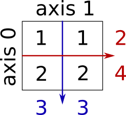 ### 1.3.2.2 基礎簡化 #### 1.3.2.2.1 計算求和 In?[79]: ``` x = np.array([1, 2, 3, 4]) np.sum(x) ``` Out[79]: ``` 10 ``` In?[80]: ``` x.sum() ``` Out[80]: ``` 10 ``` 行求和和列求和： ![reductions](http://scipy-lectures.github.io/_images/reductions.png) In?[81]: ``` x = np.array([[1, 1], [2, 2]]) x ``` Out[81]: ``` array([[1, 1], [2, 2]]) ``` In?[83]: ``` x.sum(axis=0) # 列 (第一緯度) ``` Out[83]: ``` array([3, 3]) ``` In?[84]: ``` x[:, 0].sum(), x[:, 1].sum() ``` Out[84]: ``` (3, 3) ``` In?[85]: ``` x.sum(axis=1) # 行 (第二緯度) ``` Out[85]: ``` array([2, 4]) ``` In?[86]: ``` x[0, :].sum(), x[1, :].sum() ``` Out[86]: ``` (2, 4) ``` 相同的思路在高維： In?[87]: ``` x = np.random.rand(2, 2, 2) x.sum(axis=2)[0, 1] ``` Out[87]: ``` 1.2671177193964822 ``` In?[88]: ``` x[0, 1, :].sum() ``` Out[88]: ``` 1.2671177193964822 ``` #### 1.3.2.2.2 其他簡化 * 以相同方式運作（也可以使用 `axis=` ） **極值** In?[89]: ``` x = np.array([1, 3, 2]) x.min() ``` Out[89]: ``` 1 ``` In?[90]: ``` x.max() ``` Out[90]: ``` 3 ``` In?[91]: ``` x.argmin() # 最小值的索引 ``` Out[91]: ``` 0 ``` In?[92]: ``` x.argmax() # 最大值的索引 ``` Out[92]: ``` 1 ``` **邏輯運算**： In?[93]: ``` np.all([True, True, False]) ``` Out[93]: ``` False ``` In?[94]: ``` np.any([True, True, False]) ``` Out[94]: ``` True ``` **注**：可以被應用數組對比： In?[95]: ``` a = np.zeros((100, 100)) np.any(a != 0) ``` Out[95]: ``` False ``` In?[96]: ``` np.all(a == a) ``` Out[96]: ``` True ``` In?[97]: ``` a = np.array([1, 2, 3, 2]) b = np.array([2, 2, 3, 2]) c = np.array([6, 4, 4, 5]) ((a <= b) & (b <= c)).all() ``` Out[97]: ``` True ``` **統計:** In?[98]: ``` x = np.array([1, 2, 3, 1]) y = np.array([[1, 2, 3], [5, 6, 1]]) x.mean() ``` Out[98]: ``` 1.75 ``` In?[99]: ``` np.median(x) ``` Out[99]: ``` 1.5 ``` In?[100]: ``` np.median(y, axis=-1) # 最后的坐標軸 ``` Out[100]: ``` array([ 2., 5.]) ``` In?[101]: ``` x.std() # 全體總體的標準差。 ``` Out[101]: ``` 0.82915619758884995 ``` ... 以及其他更多（隨著你成長最好學習一下）。 **練習：簡化** * 假定有 `sum` ，你會期望看到哪些其他的函數？ * `sum` 和 `cumsum` 有什么區別？ **實例: 數據統計** [populations.txt](http://scipy-lectures.github.io/_downloads/populations.txt)中的數據描述了過去20年加拿大北部野兔和猞猁的數量（以及胡蘿卜）。你可以在編輯器或在IPython看一下數據（shell或者notebook都可以）： In?[104]: ``` cat data/populations.txt ``` ``` # year hare lynx carrot 1900 30e3 4e3 48300 1901 47.2e3 6.1e3 48200 1902 70.2e3 9.8e3 41500 1903 77.4e3 35.2e3 38200 1904 36.3e3 59.4e3 40600 1905 20.6e3 41.7e3 39800 1906 18.1e3 19e3 38600 1907 21.4e3 13e3 42300 1908 22e3 8.3e3 44500 1909 25.4e3 9.1e3 42100 1910 27.1e3 7.4e3 46000 1911 40.3e3 8e3 46800 1912 57e3 12.3e3 43800 1913 76.6e3 19.5e3 40900 1914 52.3e3 45.7e3 39400 1915 19.5e3 51.1e3 39000 1916 11.2e3 29.7e3 36700 1917 7.6e3 15.8e3 41800 1918 14.6e3 9.7e3 43300 1919 16.2e3 10.1e3 41300 1920 24.7e3 8.6e3 47300 ``` 首先，將數據加載到Numpy數組： In?[107]: ``` data = np.loadtxt('data/populations.txt') year, hares, lynxes, carrots = data.T # 技巧: 將列分配給變量 ``` 接下來作圖： In?[108]: ``` from matplotlib import pyplot as plt plt.axes([0.2, 0.1, 0.5, 0.8]) plt.plot(year, hares, year, lynxes, year, carrots) plt.legend(('Hare', 'Lynx', 'Carrot'), loc=(1.05, 0.5)) ``` Out[108]: ``` <matplotlib.legend.Legend at 0x1070407d0> ``` ![](https://box.kancloud.cn/2016-03-21_56efdc070e4c1.png) 隨時間變化的人口平均數： In?[109]: ``` populations = data[:, 1:] populations.mean(axis=0) ``` Out[109]: ``` array([ 34080.95238095, 20166.66666667, 42400\. ]) ``` 樣本的標準差： In?[110]: ``` populations.std(axis=0) ``` Out[110]: ``` array([ 20897.90645809, 16254.59153691, 3322.50622558]) ``` 每一年哪個物種有最高的人口？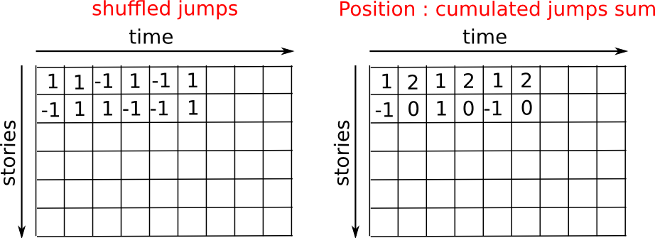： In?[111]: ``` np.argmax(populations, axis=1) ``` Out[111]: ``` array([2, 2, 0, 0, 1, 1, 2, 2, 2, 2, 2, 2, 0, 0, 0, 1, 2, 2, 2, 2, 2]) ``` **實例：隨機游走算法擴散** [random_walk](http://scipy-lectures.github.io/_images/random_walk.png) 讓我們考慮一下簡單的1維隨機游走過程：在每個時間點，行走者以相等的可能性跳到左邊或右邊。我們感興趣的是找到隨機游走者在 `t` 次左跳或右跳后距離原點的典型距離？我們將模擬許多”行走者“來找到這個規律，并且我們將采用數組計算技巧來計算：我們將創建一個2D數組記錄事實，一個方向是經歷（每個行走者有一個經歷），一個緯度是時間： ![random_walk_schema](http://scipy-lectures.github.io/_images/random_walk_schema.png) In?[113]: ``` n_stories = 1000 # 行走者的數 t_max = 200 # 我們跟蹤行走者的時間 ``` 我們隨機選擇步長1或-1去行走： In?[115]: ``` t = np.arange(t_max) steps = 2 * np.random.random_integers(0, 1, (n_stories, t_max)) - 1 np.unique(steps) # 驗證: 所有步長是1或-1 ``` Out[115]: ``` array([-1, 1]) ``` 我們通過匯總隨著時間的步驟來構建游走 In?[116]: ``` positions = np.cumsum(steps, axis=1) # axis = 1: 緯度是時間 sq_distance = positions**2 ``` 獲得經歷軸的平均數： In?[117]: ``` mean_sq_distance = np.mean(sq_distance, axis=0) ``` 畫出結果： In?[126]: ``` plt.figure(figsize=(4, 3)) plt.plot(t, np.sqrt(mean_sq_distance), 'g.', t, np.sqrt(t), 'y-') plt.xlabel(r"$t$") plt.ylabel(r"$\sqrt{\langle (\delta x)^2 \rangle}$") ``` Out[126]: ``` <matplotlib.text.Text at 0x10b529450> ``` ![](https://box.kancloud.cn/2016-03-21_56efdc0722348.png) 我們找到了物理學上一個著名的結果：均方差記錄是時間的平方根！ ### 1.3.2.3 廣播 * numpy數組的基本操作（相加等）是元素級別的 * 在相同大小的數組上仍然適用。 **盡管如此**, 也可能在不同大小的數組上進行這個操作，假如Numpy可以將這些數組轉化為相同的大小：這種轉化稱為廣播。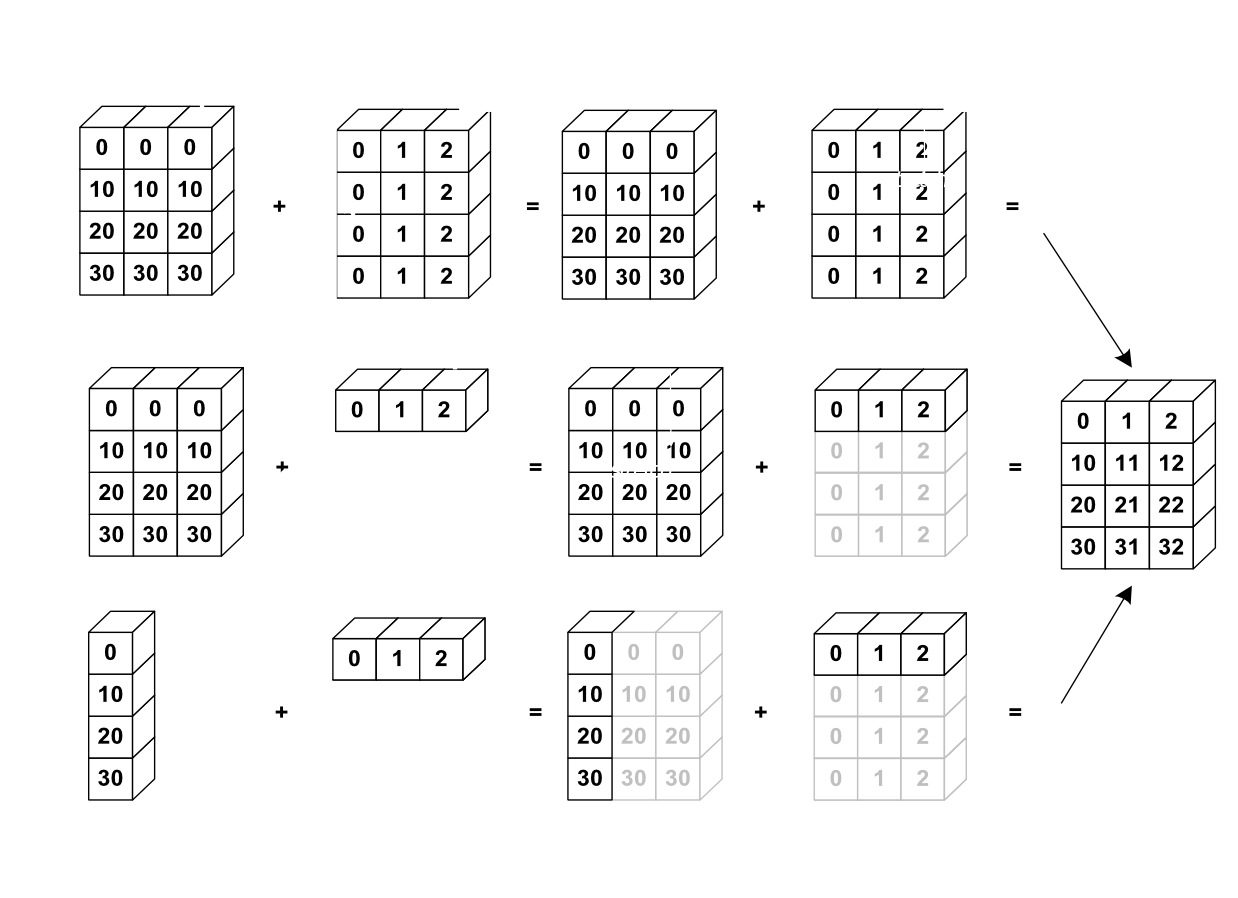下圖給出了一個廣播的例子： ![numpy_broadcasting](http://scipy-lectures.github.io/_images/numpy_broadcasting.png) 讓我們驗證一下： In?[127]: ``` a = np.tile(np.arange(0, 40, 10), (3, 1)).T a ``` Out[127]: ``` array([[ 0, 0, 0], [10, 10, 10], [20, 20, 20], [30, 30, 30]]) ``` In?[128]: ``` b = np.array([0, 1, 2]) a + b ``` Out[128]: ``` array([[ 0, 1, 2], [10, 11, 12], [20, 21, 22], [30, 31, 32]]) ``` 在不知道廣播的時候已經使用過它！： In?[129]: ``` a = np.ones((4, 5)) a[0] = 2 # 我們將一個數組的緯度0分配給另一個數組的緯度1 a ``` Out[129]: ``` array([[ 2., 2., 2., 2., 2.], [ 1., 1., 1., 1., 1.], [ 1., 1., 1., 1., 1.], [ 1., 1., 1., 1., 1.]]) ``` In?[130]: ``` a = np.ones((4, 5)) print a[0] a[0] = 2 # 我們將一個數組的緯度0分配給另一個數組的緯度 a ``` ``` [ 1\. 1\. 1\. 1\. 1.] ``` Out[130]: ``` array([[ 2., 2., 2., 2., 2.], [ 1., 1., 1., 1., 1.], [ 1., 1., 1., 1., 1.], [ 1., 1., 1., 1., 1.]]) ``` 一個有用的技巧： In?[133]: ``` a = np.arange(0, 40, 10) a.shape ``` Out[133]: ``` (4,) ``` In?[134]: ``` a = a[:, np.newaxis] # 添加一個新的軸 -> 2D 數組 a.shape ``` Out[134]: ``` (4, 1) ``` In?[135]: ``` a ``` Out[135]: ``` array([[ 0], [10], [20], [30]]) ``` In?[136]: ``` a + b ``` Out[136]: ``` array([[ 0, 1, 2], [10, 11, 12], [20, 21, 22], [30, 31, 32]]) ``` 廣播看起來很神奇，但是，當我們要解決的問題是輸出數據比輸入數據有更多緯度的數組時，使用它是非常自然的。 **實例：廣播** 讓我們創建一個66號公路上城市之間距離（用公里計算）的數組：芝加哥、斯普林菲爾德、圣路易斯、塔爾薩、俄克拉何馬市、阿馬里洛、圣塔菲、阿爾布開克、Flagstaff、洛杉磯。 In?[138]: ``` mileposts = np.array([0, 198, 303, 736, 871, 1175, 1475, 1544, 1913, 2448]) distance_array = np.abs(mileposts - mileposts[:, np.newaxis]) distance_array ``` Out[138]: ``` array([[ 0, 198, 303, 736, 871, 1175, 1475, 1544, 1913, 2448], [ 198, 0, 105, 538, 673, 977, 1277, 1346, 1715, 2250], [ 303, 105, 0, 433, 568, 872, 1172, 1241, 1610, 2145], [ 736, 538, 433, 0, 135, 439, 739, 808, 1177, 1712], [ 871, 673, 568, 135, 0, 304, 604, 673, 1042, 1577], [1175, 977, 872, 439, 304, 0, 300, 369, 738, 1273], [1475, 1277, 1172, 739, 604, 300, 0, 69, 438, 973], [1544, 1346, 1241, 808, 673, 369, 69, 0, 369, 904], [1913, 1715, 1610, 1177, 1042, 738, 438, 369, 0, 535], [2448, 2250, 2145, 1712, 1577, 1273, 973, 904, 535, 0]]) ``` ![route66](http://scipy-lectures.github.io/_images/route66.png) 許多基于網格或者基于網絡的問題都需要使用廣播。例如，如果要計算10X10網格中每個點到原點的數據，可以這樣： In?[139]: ``` x, y = np.arange(5), np.arange(5)[:, np.newaxis] distance = np.sqrt(x ** 2 + y ** 2) distance ``` Out[139]: ``` array([[ 0\. , 1\. , 2\. , 3\. , 4\. ], [ 1\. , 1.41421356, 2.23606798, 3.16227766, 4.12310563], [ 2\. , 2.23606798, 2.82842712, 3.60555128, 4.47213595], [ 3\. , 3.16227766, 3.60555128, 4.24264069, 5\. ], [ 4\. , 4.12310563, 4.47213595, 5\. , 5.65685425]]) ``` 或者用顏色： In?[141]: ``` plt.pcolor(distance) plt.colorbar() ``` Out[141]: ``` <matplotlib.colorbar.Colorbar instance at 0x10d8d7170> ``` ![](https://box.kancloud.cn/2016-03-21_56efdc07320c2.png) **評論** : `numpy.ogrid` 函數允許直接創建上一個例子中兩個**重要緯度**向量X和Y： In?[142]: ``` x, y = np.ogrid[0:5, 0:5] x, y ``` Out[142]: ``` (array([[0], [1], [2], [3], [4]]), array([[0, 1, 2, 3, 4]])) ``` In?[143]: ``` x.shape, y.shape ``` Out[143]: ``` ((5, 1), (1, 5)) ``` In?[144]: ``` distance = np.sqrt(x ** 2 + y ** 2) ``` 因此， `np.ogrid` 就非常有用，只要我們是要處理網格計算。另一方面，在一些無法（或者不想）從廣播中收益的情況下，`np.mgrid` 直接提供了由索引構成的矩陣： In?[145]: ``` x, y = np.mgrid[0:4, 0:4] x ``` Out[145]: ``` array([[0, 0, 0, 0], [1, 1, 1, 1], [2, 2, 2, 2], [3, 3, 3, 3]]) ``` In?[146]: ``` y ``` Out[146]: ``` array([[0, 1, 2, 3], [0, 1, 2, 3], [0, 1, 2, 3], [0, 1, 2, 3]]) ``` ### 1.3.2.4數組形狀操作 #### 1.3.2.4.1 扁平 In?[147]: ``` a = np.array([[1, 2, 3], [4, 5, 6]]) a.ravel() ``` Out[147]: ``` array([1, 2, 3, 4, 5, 6]) ``` In?[148]: ``` a.T ``` Out[148]: ``` array([[1, 4], [2, 5], [3, 6]]) ``` In?[149]: ``` a.T.ravel() ``` Out[149]: ``` array([1, 4, 2, 5, 3, 6]) ``` 高維：后進先出。 #### 1.3.2.4.2 重排扁平的相反操作： In?[150]: ``` a.shape ``` Out[150]: ``` (2, 3) ``` In?[152]: ``` b = a.ravel() b = b.reshape((2, 3)) b ``` Out[152]: ``` array([[1, 2, 3], [4, 5, 6]]) ``` 或者： In?[153]: ``` a.reshape((2, -1)) # 不確定的值（-1）將被推導 ``` Out[153]: ``` array([[1, 2, 3], [4, 5, 6]]) ``` **警告**： `ndarray.reshape` 可以返回一個視圖（參見 `help(np.reshape)`）, 也可以可以返回副本 In?[155]: ``` b[0, 0] = 99 a ``` Out[155]: ``` array([[99, 2, 3], [ 4, 5, 6]]) ``` 當心：重排也可以返回一個副本！： In?[156]: ``` a = np.zeros((3, 2)) b = a.T.reshape(3*2) b[0] = 9 a ``` Out[156]: ``` array([[ 0., 0.], [ 0., 0.], [ 0., 0.]]) ``` 要理解這個現象，你需要了解更多關于numpy數組內存設計的知識。 #### 1.3.2.4.3 添加緯度用 `np.newaxis`對象進行索引可以為一個數組添加軸（在上面關于廣播的部分你已經看到過了）： In?[157]: ``` z = np.array([1, 2, 3]) z ``` Out[157]: ``` array([1, 2, 3]) ``` In?[158]: ``` z[:, np.newaxis] ``` Out[158]: ``` array([[1], [2], [3]]) ``` In?[159]: ``` z[np.newaxis, :] ``` Out[159]: ``` array([[1, 2, 3]]) ``` #### 1.3.2.4.4 緯度重組 In?[160]: ``` a = np.arange(4*3*2).reshape(4, 3, 2) a.shape ``` Out[160]: ``` (4, 3, 2) ``` In?[161]: ``` a[0, 2, 1] ``` Out[161]: ``` 5 ``` In?[163]: ``` b = a.transpose(1, 2, 0) b.shape ``` Out[163]: ``` (3, 2, 4) ``` In?[164]: ``` b[2, 1, 0] ``` Out[164]: ``` 5 ``` 也是創建了一個視圖： In?[165]: ``` b[2, 1, 0] = -1 a[0, 2, 1] ``` Out[165]: ``` -1 ``` #### 1.3.2.4.5 改變大小可以用 `ndarray.resize` 改變數組的大小： In?[167]: ``` a = np.arange(4) a.resize((8,)) a ``` Out[167]: ``` array([0, 1, 2, 3, 0, 0, 0, 0]) ``` 但是，它不能在其他地方引用： In?[168]: ``` b = a a.resize((4,)) ``` ``` --------------------------------------------------------------------------- ValueError Traceback (most recent call last) <ipython-input-168-59edd3107605> in <module>() 1 b = a ----> 2 a.resize((4,)) ValueError: cannot resize an array that references or is referenced by another array in this way. Use the resize function ``` **練習：形狀操作** * 看一下 `reshape` 的文檔字符串，特別要注意其中關于副本和視圖的內容。 * 用 `flatten` 來替換 `ravel`。有什么區別？ (提示: 試一下哪個返回視圖哪個返回副本) * 試一下用 `transpose` 來進行緯度變換。 ### 1.3.2.5 數據排序按一個軸排序： In?[169]: ``` a = np.array([[4, 3, 5], [1, 2, 1]]) b = np.sort(a, axis=1) b ``` Out[169]: ``` array([[3, 4, 5], [1, 1, 2]]) ``` **注**：每行分別排序！原地排序： In?[170]: ``` a.sort(axis=1) a ``` Out[170]: ``` array([[3, 4, 5], [1, 1, 2]]) ``` 象征索引排序： In?[171]: ``` a = np.array([4, 3, 1, 2]) j = np.argsort(a) j ``` Out[171]: ``` array([2, 3, 1, 0]) ``` In?[172]: ``` a[j] ``` Out[172]: ``` array([1, 2, 3, 4]) ``` 找到最大值和最小值： In?[173]: ``` a = np.array([4, 3, 1, 2]) j_max = np.argmax(a) j_min = np.argmin(a) j_max, j_min ``` Out[173]: ``` (0, 2) ``` **練習：排序** * 試一下原地和非原地排序 * 試一下用不同的數據類型創建數組并且排序。 * 用 `all` 或者 `array_equal` 來檢查一下結果。 * 看一下 `np.random.shuffle`，一種更快創建可排序輸入的方式。 * 合并 `ravel` 、`sort` 和 `reshape`。 * 看一下 `sort` 的 `axis` 關鍵字，重寫一下這個練習。 ### 1.3.2.6 總結 **入門你需要了解什么？** * 了解如何創建數組：`array`、`arange`、`ones`、`zeros`。 * 了解用 `array.shape`數組的形狀，然后使用切片來獲得數組的不同視圖：`array[::2]`等。用 `reshape`改變數組形狀或者用 `ravel`扁平化。 * 獲得數組元素的一個子集，和/或用面具修改他們的值ay and/or modify their values with masks In?[174]: ``` a[a < 0] = 0 ``` * 了解數組上各式各樣的操作，比如找到平均數或最大值 (`array.max()`、`array.mean()`)。不需要記住所有東西，但是應該有條件反射去搜索文檔 (線上文檔, `help()`, `lookfor()`)!! * 更高級的用法：掌握用整型數組索引，以及廣播。了解更多的Numpy函數以便處理多種數組操作。 **快讀閱讀** 如果你想要快速通過科學講座筆記來學習生態系統，你可以直接跳到下一章：Matplotlib: 作圖(暫缺)。本章剩下的內容對于學習介紹部分不是必須的。但是，記得回來完成本章并且完成更多的練習。 ## 1.3.3 數據的更多內容 ### 1.3.3.1 更多的數據類型 #### 1.3.3.1.1 投射 “更大”的類型在混合類型操作中勝出： In?[175]: ``` np.array([1, 2, 3]) + 1.5 ``` Out[175]: ``` array([ 2.5, 3.5, 4.5]) ``` 賦值不會改變類型！ In?[176]: ``` a = np.array([1, 2, 3]) a.dtype ``` Out[176]: ``` dtype('int64') ``` In?[178]: ``` a[0] = 1.9 # <-- 浮點被截取為整數 a ``` Out[178]: ``` array([1, 2, 3]) ``` 強制投射： In?[179]: ``` a = np.array([1.7, 1.2, 1.6]) b = a.astype(int) # <-- 截取整數 b ``` Out[179]: ``` array([1, 1, 1]) ``` 四舍五入： In?[180]: ``` a = np.array([1.2, 1.5, 1.6, 2.5, 3.5, 4.5]) b = np.around(a) b # 仍然是浮點 ``` Out[180]: ``` array([ 1., 2., 2., 2., 4., 4.]) ``` In?[181]: ``` c = np.around(a).astype(int) c ``` Out[181]: ``` array([1, 2, 2, 2, 4, 4]) ``` #### 1.3.3.1.2 不同數據類型的大小整數 (帶有符號): | 類型 | 字節數 | | --- | --- | | int8 | 8 bits | | int16 | 16 bits | | int32 | 32 bits (與32位平臺的int相同) | | int64 | 64 bits (與64位平臺的int相同) | In?[182]: ``` np.array([1], dtype=int).dtype ``` Out[182]: ``` dtype('int64') ``` In?[183]: ``` np.iinfo(np.int32).max, 2**31 - 1 ``` Out[183]: ``` (2147483647, 2147483647) ``` In?[184]: ``` np.iinfo(np.int64).max, 2**63 - 1 ``` Out[184]: ``` (9223372036854775807, 9223372036854775807L) ``` 無符號整數: | 類型 | 字節數 | | --- | --- | | uint8 | 8 bits | | uint16 | 16 bits | | uint32 | 32 bits | | uint64 | 64 bits | In?[185]: ``` np.iinfo(np.uint32).max, 2**32 - 1 ``` Out[185]: ``` (4294967295, 4294967295) ``` In?[186]: ``` np.iinfo(np.uint64).max, 2**64 - 1 ``` Out[186]: ``` (18446744073709551615L, 18446744073709551615L) ``` 浮點數據： | 類型 | 字節數 | | --- | --- | | float16 | 16 bits | | float32 | 32 bits | | float64 | 64 bits (與浮點相同) | | float96 | 96 bits, 平臺依賴 (與 `np.longdouble` 相同) | | float128 | 128 bits, 平臺依賴 (與 `np.longdouble`相同) | In?[187]: ``` np.finfo(np.float32).eps ``` Out[187]: ``` 1.1920929e-07 ``` In?[188]: ``` np.finfo(np.float64).eps ``` Out[188]: ``` 2.2204460492503131e-16 ``` In?[189]: ``` np.float32(1e-8) + np.float32(1) == 1 ``` Out[189]: ``` True ``` In?[190]: ``` np.float64(1e-8) + np.float64(1) == 1 ``` Out[190]: ``` False ``` 浮點復數： | 類型 | 字節數 | | --- | --- | | complex64 | 兩個 32-bit 浮點 | | complex128 | 兩個 64-bit 浮點 | | complex192 | 兩個 96-bit 浮點, 平臺依賴 | | complex256 | 兩個 128-bit 浮點, 平臺依賴 | **更小的數據類型** 如果你不知道需要特殊數據類型，那你可能就不需要。比較使用 `float32`代替 `float64`: * 一半的內存和硬盤大小 * 需要一半的寬帶（可能在一些操作中更快） In?[191]: ``` a = np.zeros((1e6,), dtype=np.float64) b = np.zeros((1e6,), dtype=np.float32) %timeit a*a ``` ``` 1000 loops, best of 3: 1.41 ms per loop ``` In?[192]: ``` %timeit b*b ``` ``` 1000 loops, best of 3: 739 μs per loop ``` * 但是更大的四舍五入誤差 - 有時在一些令人驚喜的地方（即，不要使用它們除非你真的需要） ### 1.3.3.2 結構化的數據類型 | 名稱 | 類型 | | --- | --- | | sensor_code | (4個字母的字符) | | position | (浮點) | | value | (浮點) | In?[194]: ``` samples = np.zeros((6,), dtype=[('sensor_code', 'S4'),('position', float), ('value', float)]) samples.ndim ``` Out[194]: ``` 1 ``` In?[195]: ``` samples.shape ``` Out[195]: ``` (6,) ``` In?[196]: ``` samples.dtype.names ``` Out[196]: ``` ('sensor_code', 'position', 'value') ``` In?[198]: ``` samples[:] = [('ALFA', 1, 0.37), ('BETA', 1, 0.11), ('TAU', 1, 0.13),('ALFA', 1.5, 0.37), ('ALFA', 3, 0.11), ('TAU', 1.2, 0.13)] samples ``` Out[198]: ``` array([('ALFA', 1.0, 0.37), ('BETA', 1.0, 0.11), ('TAU', 1.0, 0.13), ('ALFA', 1.5, 0.37), ('ALFA', 3.0, 0.11), ('TAU', 1.2, 0.13)], dtype=[('sensor_code', 'S4'), ('position', '<f8'), ('value', '<f8')]) ``` 用字段名稱索引也可以訪問字段： In?[199]: ``` samples['sensor_code'] ``` Out[199]: ``` array(['ALFA', 'BETA', 'TAU', 'ALFA', 'ALFA', 'TAU'], dtype='|S4') ``` In?[200]: ``` samples['value'] ``` Out[200]: ``` array([ 0.37, 0.11, 0.13, 0.37, 0.11, 0.13]) ``` In?[201]: ``` samples[0] ``` Out[201]: ``` ('ALFA', 1.0, 0.37) ``` In?[202]: ``` samples[0]['sensor_code'] = 'TAU' samples[0] ``` Out[202]: ``` ('TAU', 1.0, 0.37) ``` 一次多個字段： In?[203]: ``` samples[['position', 'value']] ``` Out[203]: ``` array([(1.0, 0.37), (1.0, 0.11), (1.0, 0.13), (1.5, 0.37), (3.0, 0.11), (1.2, 0.13)], dtype=[('position', '<f8'), ('value', '<f8')]) ``` 和普通情況一樣，象征索引也有效： In?[204]: ``` samples[samples['sensor_code'] == 'ALFA'] ``` Out[204]: ``` array([('ALFA', 1.5, 0.37), ('ALFA', 3.0, 0.11)], dtype=[('sensor_code', 'S4'), ('position', '<f8'), ('value', '<f8')]) ``` **注**：構建結構化數組有需要其他的語言，見[這里](http://docs.scipy.org/doc/numpy/user/basics.rec.html)和[這里](http://docs.scipy.org/doc/numpy/reference/arrays.dtypes.html#specifying-and-constructing-data-types)。 ### 1.3.3.3 面具數組（maskedarray）: 處理缺失值（的傳播） * 對于浮點不能用NaN，但是面具對所有類型都適用： In?[207]: ``` x = np.ma.array([1, 2, 3, 4], mask=[0, 1, 0, 1]) x ``` Out[207]: ``` masked_array(data = [1 -- 3 --], mask = [False True False True], fill_value = 999999) ``` In?[208]: ``` y = np.ma.array([1, 2, 3, 4], mask=[0, 1, 1, 1]) x + y ``` Out[208]: ``` masked_array(data = [2 -- -- --], mask = [False True True True], fill_value = 999999) ``` * 通用函數的面具版本： In?[209]: ``` np.ma.sqrt([1, -1, 2, -2]) ``` Out[209]: ``` masked_array(data = [1.0 -- 1.4142135623730951 --], mask = [False True False True], fill_value = 1e+20) ``` **注**：有許多其他數組的[兄弟姐妹](http://scipy-lectures.github.io/advanced/advanced_numpy/index.html#array-siblings) 盡管這脫離了Numpy這章的主題，讓我們花點時間回憶一下編寫代碼的最佳實踐，從長遠角度這絕對是值得的： **最佳實踐** * 明確的變量名（不需要備注去解釋變量里是什么） * 風格：逗號后及＝周圍有空格等。在[Python代碼風格指南](http://www.python.org/dev/peps/pep-0008)及[文檔字符串慣例](http://www.python.org/dev/peps/pep-0257)頁面中給出了相當數據量如何書寫“漂亮代碼”的規則（并且，最重要的是，與其他人使用相同的慣例!）。 * 除非在一些及特殊的情況下，變量名及備注用英文。 ## 1.3.4 高級操作 1.3.4.1\. 多項式 Numpy也包含不同基的多項式：例如，$3x^2 + 2x - 1$: In?[211]: ``` p = np.poly1d([3, 2, -1]) p(0) ``` Out[211]: ``` -1 ``` In?[212]: ``` p.roots ``` Out[212]: ``` array([-1\. , 0.33333333]) ``` In?[213]: ``` p.order ``` Out[213]: ``` 2 ``` In?[215]: ``` x = np.linspace(0, 1, 20) y = np.cos(x) + 0.3*np.random.rand(20) p = np.poly1d(np.polyfit(x, y, 3)) t = np.linspace(0, 1, 200) plt.plot(x, y, 'o', t, p(t), '-') ``` Out[215]: ``` [<matplotlib.lines.Line2D at 0x10f40c2d0>, <matplotlib.lines.Line2D at 0x10f40c510>] ``` ![](https://box.kancloud.cn/2016-03-21_56efdc0742c3c.png) 更多內容見[http://docs.scipy.org/doc/numpy/reference/routines.polynomials.poly1d.html。](http://docs.scipy.org/doc/numpy/reference/routines.polynomials.poly1d.html。) #### 1.3.4.1.1 更多多項式（有更多的基） Numpy也有更復雜的多項式接口，支持比如切比雪夫基。 $3x^2 + 2x - 1$: In?[216]: ``` p = np.polynomial.Polynomial([-1, 2, 3]) # 系數的順序不同！ p(0) ``` Out[216]: ``` -1.0 ``` In?[217]: ``` p.roots() ``` Out[217]: ``` array([-1\. , 0.33333333]) ``` In?[218]: ``` p.degree() # 在普通的多項式中通常不暴露'order' ``` Out[218]: ``` 2 ``` 在切爾雪夫基中使用多項式的例子，多項式的范圍在[-1,1]： In?[221]: ``` x = np.linspace(-1, 1, 2000) y = np.cos(x) + 0.3*np.random.rand(2000) p = np.polynomial.Chebyshev.fit(x, y, 90) t = np.linspace(-1, 1, 200) plt.plot(x, y, 'r.') plt.plot(t, p(t), 'k-', lw=3) ``` Out[221]: ``` [<matplotlib.lines.Line2D at 0x10f442d10>] ``` ![](https://box.kancloud.cn/2016-03-21_56efdc0751c7d.png) 切爾雪夫多項式在插入方面有很多優勢。 ### 1.3.4.2 加載數據文件 #### 1.3.4.2.1 文本文件例子: [populations.txt](http://scipy-lectures.github.io/_downloads/populations.txt): ``` # year hare lynx carrot 1900 30e3 4e3 48300 1901 47.2e3 6.1e3 48200 1902 70.2e3 9.8e3 41500 1903 77.4e3 35.2e3 38200 ``` In?[222]: ``` data = np.loadtxt('data/populations.txt') data ``` Out[222]: ``` array([[ 1900., 30000., 4000., 48300.], [ 1901., 47200., 6100., 48200.], [ 1902., 70200., 9800., 41500.], [ 1903., 77400., 35200., 38200.], [ 1904., 36300., 59400., 40600.], [ 1905., 20600., 41700., 39800.], [ 1906., 18100., 19000., 38600.], [ 1907., 21400., 13000., 42300.], [ 1908., 22000., 8300., 44500.], [ 1909., 25400., 9100., 42100.], [ 1910., 27100., 7400., 46000.], [ 1911., 40300., 8000., 46800.], [ 1912., 57000., 12300., 43800.], [ 1913., 76600., 19500., 40900.], [ 1914., 52300., 45700., 39400.], [ 1915., 19500., 51100., 39000.], [ 1916., 11200., 29700., 36700.], [ 1917., 7600., 15800., 41800.], [ 1918., 14600., 9700., 43300.], [ 1919., 16200., 10100., 41300.], [ 1920., 24700., 8600., 47300.]]) ``` In?[224]: ``` np.savetxt('pop2.txt', data) data2 = np.loadtxt('pop2.txt') ``` **注**：如果你有一個復雜的文本文件，應該嘗試： * `np.genfromtxt` * 使用Python的I/O函數和例如正則式來解析（Python特別適合這個工作） **提示：用IPython在文件系統中航行** In?[225]: ``` pwd # 顯示當前目錄 ``` Out[225]: ``` u'/Users/cloga/Documents/scipy-lecture-notes_cn' ``` In?[227]: ``` cd data ``` ``` /Users/cloga/Documents/scipy-lecture-notes_cn/data ``` In?[228]: ``` ls ``` ``` populations.txt ``` #### 1.3.4.2.2 圖像使用Matplotlib： In?[233]: ``` img = plt.imread('data/elephant.png') img.shape, img.dtype ``` Out[233]: ``` ((200, 300, 3), dtype('float32')) ``` In?[234]: ``` plt.imshow(img) ``` Out[234]: ``` <matplotlib.image.AxesImage at 0x10fd13f10> ``` ![](https://box.kancloud.cn/2016-03-21_56efdc0763bd7.png) In?[237]: ``` plt.savefig('plot.png') plt.imsave('red_elephant', img[:,:,0], cmap=plt.cm.gray) ``` ``` <matplotlib.figure.Figure at 0x10fba1750> ``` 這只保存了一個渠道（RGB）： In?[238]: ``` plt.imshow(plt.imread('red_elephant.png')) ``` Out[238]: ``` <matplotlib.image.AxesImage at 0x11040e150> ``` ![](https://box.kancloud.cn/2016-03-21_56efdc078718d.png) 其他包： In?[239]: ``` from scipy.misc import imsave imsave('tiny_elephant.png', img[::6,::6]) plt.imshow(plt.imread('tiny_elephant.png'), interpolation='nearest') ``` Out[239]: ``` <matplotlib.image.AxesImage at 0x110bfbfd0> ``` ![](https://box.kancloud.cn/2016-03-21_56efdc07a8b32.png) #### 1.3.4.2.3 Numpy的自有格式 Numpy有自有的二進制格式，沒有便攜性但是I/O高效： In?[240]: ``` data = np.ones((3, 3)) np.save('pop.npy', data) data3 = np.load('pop.npy') ``` #### 1.3.4.2.4 知名的（并且更復雜的）文件格式 * HDF5: [h5py](http://code.google.com/p/h5py/), [PyTables](http://pytables.org/) * NetCDF: `scipy.io.netcdf_file`, [netcdf4-python](http://code.google.com/p/netcdf4-python/), ... * Matlab: `scipy.io.loadmat`, `scipy.io.savemat` * MatrixMarket: `scipy.io.mmread`, `scipy.io.mmread` ... 如果有人使用，那么就可能有一個對應的Python庫。 **練習：文本數據文件** 寫一個Python腳本從[populations.txt](http://scipy-lectures.github.io/_downloads/populations.txt)加載數據，刪除前五行和后五行。將這個小數據集存入 `pop2.txt`。 **Numpy內部** 如果你對Numpy的內部感興趣, 有一個關于[Advanced Numpy](http://scipy-lectures.github.io/advanced/advanced_numpy/index.html#advanced-numpy)的很好的討論。 ## 1.3.5 一些練習 ### 1.3.5.1 數組操作 * 從2D數組（不需要顯示的輸入）: ``` [[1, 6, 11], [2, 7, 12], [3, 8, 13], [4, 9, 14], [5, 10, 15]] ``` 并且生成一個第二和第四行的新數組。 * 將數組a的每一列以元素的方式除以數組b (提示: `np.newaxis`): In?[243]: ``` a = np.arange(25).reshape(5, 5) b = np.array([1., 5, 10, 15, 20]) ``` * 難一點的題目：創建10 X 3的隨機數數組（在[0, 1]的范圍內）。對于每一行，挑出最接近0.5的數。 * 用 `abs`和 `argsort`找到每一行中最接近的列 `j`。 * 使用象征索引抽取數字。（提示：a[i,j]-數組 `i` 必須包含 `j` 中成分的對應行數） ### 1.3.5.2 圖片操作：給Lena加邊框讓我們從著名的Lena圖（[http://www.cs.cmu.edu/~chuck/lennapg/）](http://www.cs.cmu.edu/~chuck/lennapg/）) 上開始，用Numpy數組做一些操作。Scipy在 `scipy.lena`函數中提供了這個圖的二維數組： In?[244]: ``` from scipy import misc lena = misc.lena() ``` **注**：在舊版的scipy中，你會在 `scipy.lena()`找到lena。這是一些通過我們的操作可以獲得圖片：使用不同的顏色地圖，裁剪圖片，改變圖片的一部分。 ![lenas](http://scipy-lectures.github.io/_images/lenas.png) * 讓我們用pylab的 `imshow`函數顯示這個圖片。 In?[245]: ``` import pylab as plt lena = misc.lena() plt.imshow(lena) ``` Out[245]: ``` <matplotlib.image.AxesImage at 0x110f51ad0> ``` ![](https://box.kancloud.cn/2016-03-21_56efdc07bf16f.png) * Lena然后以為色彩顯示。要將她展示為灰色需要指定一個顏色地圖。 In?[246]: ``` plt.imshow(lena, cmap=plt.cm.gray) ``` Out[246]: ``` <matplotlib.image.AxesImage at 0x110fb15d0> ``` ![](https://box.kancloud.cn/2016-03-21_56efdc07dea48.png) * 用一個更小的圖片中心來創建數組：例如，從圖像邊緣刪除30像素。要檢查結果，用 `imshow` 顯示這個新數組。 In?[247]: ``` crop_lena = lena[30:-30,30:-30] ``` * 現在我們為Lena的臉加一個黑色項鏈形邊框。要做到這一點，需要創建一個面具對應于需要變成黑色的像素。這個面具由如下條件定義 `(y-256)**2 + (x-256)**2` In?[248]: ``` y, x = np.ogrid[0:512,0:512] # x 和 y 像素索引 y.shape, x.shape ``` Out[248]: ``` ((512, 1), (1, 512)) ``` In?[249]: ``` centerx, centery = (256, 256) # 圖像中心 mask = ((y - centery)**2 + (x - centerx)**2) > 230**2 # 圓形 ``` 接下來我們為面具對應的圖片像素賦值為0。語句非常簡單并且直覺化： In?[253]: ``` lena[mask] = 0 plt.imshow(lena) ``` Out[253]: ``` <matplotlib.image.AxesImage at 0x113d33fd0> ``` ![](https://box.kancloud.cn/2016-03-21_56efdc08037e4.png) * 接下來：將這個練習的所有命令復制到 `lena_locket.py` 腳本中，并且在IPython中用 `%run lena_locket.py`執行這個腳本，將圓形改為橢圓。 ### 1.3.5.3 數據統計 [populations.txt](http://scipy-lectures.github.io/_downloads/populations.txt)中的數據描述了野兔和猞猁（以及胡羅比）在加拿大北部過去十年的數量： In?[254]: ``` data = np.loadtxt('data/populations.txt') year, hares, lynxes, carrots = data.T # 技巧: 列到變量 plt.axes([0.2, 0.1, 0.5, 0.8]) plt.plot(year, hares, year, lynxes, year, carrots) plt.legend(('Hare', 'Lynx', 'Carrot'), loc=(1.05, 0.5)) ``` Out[254]: ``` <matplotlib.legend.Legend at 0x1135d9510> ``` ![](https://box.kancloud.cn/2016-03-21_56efdc070e4c1.png) 根據[populations.txt](http://scipy-lectures.github.io/_downloads/populations.txt)中的數據計算并打印... 1. 每個物種在這個時間段內的數量平均數及標準差。 2. 每個物種在哪一年數量最多。 3. 每一年哪個物種數量最多。（提示：`np.array(['H', 'L', 'C'])`的`argsort` 和象征索引） 4. 哪一年數量超過50000。（提示：比較和 `np.any`） 5. 每個物種有最少數量的兩年。（提示： `argsort`、象征索引） 6. 比較（作圖）野兔和猞猁總量的變化（看一下 `help(np.gradient)`）。看一下相關（見 `help(np.corrcoef)`）。 ... 所有都不應該使用for循環。答案：[Python源文件](http://scipy-lectures.github.io/_downloads/2_2_data_statistics.py) ### 1.3.5.4 粗略積分估計寫一個函數 `f(a, b, c)` 返回$a^b - c$。組成一個24x12x6數組其中包含它值在參數范圍[0,1] x [0,1] x [0,1]。接近的3-D積分 ![math](http://scipy-lectures.github.io/_images/math/7057c0b4df82c2659d776bcdc0eb1c9e16f61f9f.png) 在這個體積之上有相同的平均數。準確的結果是![result](http://scipy-lectures.github.io/_images/math/13ff2c8691c09121c0bba41558b2ad22e55e077c.png)... - 你的相對誤差是多少？（技巧：使用元素級別的操作和廣播。你可以用 `np.ogrid` 獲得在 `np.ogrid[0:1:20j]` 范圍內的數據點。） **提醒**Python函數： In?[255]: ``` def f(a, b, c): return some_result ``` 答案：[Python源文件](http://scipy-lectures.github.io/_downloads/2_3_crude_integration.py) ### 1.3.5.5 Mandelbrot集合 ![mandelbrot](http://scipy-lectures.github.io/_images/2_4_mandelbrot.png) 寫一個腳本計算Mandelbrot分形。Mandelbrot迭代 ``` N_max = 50 some_threshold = 50 c = x + 1j*y for j in xrange(N_max): z = z**2 + c ``` 點（x, y）屬于Mandelbrot集合，如果|c| < some_threshold。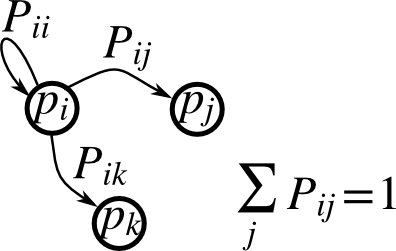作如下計算： * 構建一個網格 c = x + 1j*y，值在范圍[-2, 1] x [-1.5, 1.5] * 進行迭代 * 構建2-D布爾面具標識輸入集合中的點 * 用下列方法將結果保存到圖片： ``` import matplotlib.pyplot as plt plt.imshow(mask.T, extent=[-2, 1, -1.5, 1.5]) plt.gray() plt.savefig('mandelbrot.png') ``` 答案：[Python源文件](http://scipy-lectures.github.io/_downloads/2_4_mandelbrot.py) ### 1.3.5.6 馬爾科夫鏈 ![markov-chain](http://scipy-lectures.github.io/_images/markov-chain.png) 馬爾可夫鏈過渡矩陣P以及在狀態p的概率分布： 1. `0 <= P[i,j] <= 1`：從狀態i變化到j的概率 2. 過度規則： $p_{new} = P^T p_{old}$ 3. `all(sum(P, axis=1) == 1)`, `p.sum() == 1`: 正態化寫一個腳本產生五種狀態，并且： * 構建一個隨機矩陣，正態化每一行，以便它是過度矩陣。 * 從一個隨機（正態化）概率分布`p`開始，并且進行50步=> `p_50` * 計算穩定分布：P.T的特征值為1的特征向量（在數字上最接近1）=> `p_stationary` 記住正態化向量 - 我并沒有... * 檢查一下 `p_50` 和 `p_stationary`是否等于公差1e-5 工具箱：`np.random.rand`、 `.dot()`、`np.linalg.eig`、reductions、`abs()`、`argmin`、comparisons、`all`、`np.linalg.norm`等。答案：[Python源文件](http://scipy-lectures.github.io/_downloads/2_5_markov_chain.py)