
# 1.5 Scipy:高級科學計算
作者:Adrien Chauve, Andre Espaze, Emmanuelle Gouillart, Ga?l Varoquaux, Ralf Gommers
**Scipy**
`scipy`包包含許多專注于科學計算中的常見問題的工具箱。它的子模塊對應于不同的應用,比如插值、積分、優化、圖像處理、統計和特殊功能等。
`scipy`可以與其他標準科學計算包相對比,比如GSL (C和C++的GNU科學計算包), 或者Matlab的工具箱。`scipy`是Python中科學程序的核心程序包;這意味著有效的操作`numpy`數組,因此,numpy和scipy可以一起工作。
在實現一個程序前,有必要確認一下需要的數據處理時候已經在scipy中實現。作為非專業程序員,科學家通常傾向于**重新發明輪子**,這產生了小玩具、不優化、很難分享以及不可以維護的代碼。相反,scipy的程序是優化并且測試過的,因此應該盡可能使用。
**警告** 這個教程根本不是數值計算的介紹。因為列舉scipy的不同子模塊和功能將會是非常枯燥的,相反我們將聚焦于列出一些例子,給出如何用scipy進行科學計算的大概思路。
scipy是由針對特定任務的子模塊組成的:
| | |
| --- | --- |
| [`scipy.cluster`](http://docs.scipy.org/doc/scipy/reference/cluster.html#scipy.cluster "(in SciPy v0.13.0)") | 向量計算 / Kmeans |
| [`scipy.constants`](http://docs.scipy.org/doc/scipy/reference/constants.html#scipy.constants "(in SciPy v0.13.0)") | 物理和數學常量 |
| [`scipy.fftpack`](http://docs.scipy.org/doc/scipy/reference/fftpack.html#scipy.fftpack "(in SciPy v0.13.0)") | 傅里葉變換 |
| [`scipy.integrate`](http://docs.scipy.org/doc/scipy/reference/integrate.html#scipy.integrate "(in SciPy v0.13.0)") | 積分程序 |
| [`scipy.interpolate`](http://docs.scipy.org/doc/scipy/reference/interpolate.html#scipy.interpolate "(in SciPy v0.13.0)") | 插值 |
| [`scipy.io`](http://docs.scipy.org/doc/scipy/reference/io.html#scipy.io "(in SciPy v0.13.0)") | 數據輸入和輸出 |
| [`scipy.linalg`](http://docs.scipy.org/doc/scipy/reference/linalg.html#scipy.linalg "(in SciPy v0.13.0)") | 線性代數程序 |
| [`scipy.ndimage`](http://docs.scipy.org/doc/scipy/reference/ndimage.html#scipy.ndimage "(in SciPy v0.13.0)") | n-維圖像包 |
| [`scipy.odr`](http://docs.scipy.org/doc/scipy/reference/odr.html#scipy.odr "(in SciPy v0.13.0)") | 正交距離回歸 |
| [`scipy.optimize`](http://docs.scipy.org/doc/scipy/reference/optimize.html#scipy.optimize "(in SciPy v0.13.0)") | 優化 |
| [`scipy.signal`](http://docs.scipy.org/doc/scipy/reference/signal.html#scipy.signal "(in SciPy v0.13.0)") | 信號處理 |
| [`scipy.sparse`](http://docs.scipy.org/doc/scipy/reference/sparse.html#scipy.sparse "(in SciPy v0.13.0)") | 稀疏矩陣 |
| [`scipy.spatial`](http://docs.scipy.org/doc/scipy/reference/spatial.html#scipy.spatial "(in SciPy v0.13.0)") | 空間數據結構和算法 |
| [`scipy.special`](http://docs.scipy.org/doc/scipy/reference/special.html#scipy.special "(in SciPy v0.13.0)") | 一些特殊數學函數 |
| [`scipy.stats`](http://docs.scipy.org/doc/scipy/reference/stats.html#scipy.stats "(in SciPy v0.13.0)") | 統計 |
他們全都依賴于[numpy](http://docs.scipy.org/doc/numpy/reference/index.html#numpy), 但是大多數是彼此獨立的。導入Numpy和Scipy的標準方式:
In?[1]:
```
import numpy as np
from scipy import stats # 其他的子模塊類似
```
`scipy`的主要命名空間通常包含的函數其實是numpy(試一下`scipy.cos`其實是`np.cos`) 。這些函數的暴露只是因為歷史原因;通常沒有必要在你的代碼中使用`import scipy`。
## 1.5.1 文件輸入/輸出:[scipy.io](http://docs.scipy.org/doc/scipy/reference/io.html#scipy.io)
載入和保存matlab文件:
In?[2]:
```
from scipy import io as spio
a = np.ones((3, 3))
spio.savemat('file.mat', {'a': a}) # savemat expects a dictionary
data = spio.loadmat('file.mat', struct_as_record=True)
data['a']
```
Out[2]:
```
array([[ 1., 1., 1.],
[ 1., 1., 1.],
[ 1., 1., 1.]])
```
```
from scipy import misc
misc.imread('fname.png')
# Matplotlib也有類似的方法
import matplotlib.pyplot as plt
plt.imread('fname.png')
```
更多請見:
* 加載文本文件:[numpy.loadtxt()](http://docs.scipy.org/doc/numpy/reference/generated/numpy.loadtxt.html#numpy.loadtxt)/[numpy.savetxt()](http://docs.scipy.org/doc/numpy/reference/generated/numpy.savetxt.html#numpy.savetxt)
* 智能加載文本/csv文件:[numpy.genfromtxt()](http://docs.scipy.org/doc/numpy/reference/generated/numpy.genfromtxt.html#numpy.genfromtxt)/numpy.recfromcsv()
* 快速有效,但是針對numpy的二進制格式:[numpy.save()](http://docs.scipy.org/doc/numpy/reference/generated/numpy.save.html#numpy.save)/[numpy.load()](http://docs.scipy.org/doc/numpy/reference/generated/numpy.load.html#numpy.load)
## 1.5.2 特殊函數:[scipy.special](http://docs.scipy.org/doc/scipy/reference/special.html#scipy.special)
特殊函數是超驗函數。[scipy.special](http://docs.scipy.org/doc/scipy/reference/special.html#scipy.special)模塊的文檔字符串寫的很詳細,因此我們不會在這里列出所有的函數。常用的一些函數如下:
* 貝塞爾函數,比如`scipy.special.jn()` (第n個整型順序的貝塞爾函數)
* 橢圓函數 (`scipy.special.ellipj()` Jacobian橢圓函數, ...)
* Gamma 函數: scipy.special.gamma(), 也要注意 `scipy.special.gammaln()` 將給出更高準確數值的 Gamma的log。
* Erf, 高斯曲線的面積:scipy.special.erf()
## 1.5.3 線性代數操作:[scipy.linalg](http://docs.scipy.org/doc/scipy/reference/linalg.html#scipy.linalg)
[scipy.linalg](http://docs.scipy.org/doc/scipy/reference/linalg.html#scipy.linalg) 模塊提供了標準的線性代數操作,這依賴于底層的高效實現(BLAS、LAPACK)。
* [scipy.linalg.det()](http://docs.scipy.org/doc/scipy/reference/generated/scipy.linalg.det.html#scipy.linalg.det) 函數計算方陣的行列式:
In?[3]:
```
from scipy import linalg
arr = np.array([[1, 2],
[3, 4]])
linalg.det(arr)
```
Out[3]:
```
-2.0
```
In?[4]:
```
arr = np.array([[3, 2],
[6, 4]])
linalg.det(arr)
```
Out[4]:
```
0.0
```
In?[5]:
```
linalg.det(np.ones((3, 4)))
```
```
---------------------------------------------------------------------------
ValueError Traceback (most recent call last)
<ipython-input-5-4d4672bd00a7> in <module>()
----> 1 linalg.det(np.ones((3, 4)))
/Library/Python/2.7/site-packages/scipy/linalg/basic.pyc in det(a, overwrite_a, check_finite)
440 a1 = np.asarray(a)
441 if len(a1.shape) != 2 or a1.shape[0] != a1.shape[1]:
--> 442 raise ValueError('expected square matrix')
443 overwrite_a = overwrite_a or _datacopied(a1, a)
444 fdet, = get_flinalg_funcs(('det',), (a1,))
ValueError: expected square matrix
```
* [scipy.linalg.inv()](http://docs.scipy.org/doc/scipy/reference/generated/scipy.linalg.inv.html#scipy.linalg.inv) 函數計算逆方陣:
In?[6]:
```
arr = np.array([[1, 2],
[3, 4]])
iarr = linalg.inv(arr)
iarr
```
Out[6]:
```
array([[-2\. , 1\. ],
[ 1.5, -0.5]])
```
In?[7]:
```
np.allclose(np.dot(arr, iarr), np.eye(2))
```
Out[7]:
```
True
```
最后計算逆奇異矩陣(行列式為0)將拋出`LinAlgError` :
In?[8]:
```
arr = np.array([[3, 2],
[6, 4]])
linalg.inv(arr)
```
```
---------------------------------------------------------------------------
LinAlgError Traceback (most recent call last)
<ipython-input-8-e8078a9a17b2> in <module>()
1 arr = np.array([[3, 2],
2 [6, 4]])
----> 3 linalg.inv(arr)
/Library/Python/2.7/site-packages/scipy/linalg/basic.pyc in inv(a, overwrite_a, check_finite)
381 inv_a, info = getri(lu, piv, lwork=lwork, overwrite_lu=1)
382 if info > 0:
--> 383 raise LinAlgError("singular matrix")
384 if info < 0:
385 raise ValueError('illegal value in %d-th argument of internal '
LinAlgError: singular matrix
```
* 還有更多高級的操作,奇異值分解(SVD):
In?[9]:
```
arr = np.arange(9).reshape((3, 3)) + np.diag([1, 0, 1])
uarr, spec, vharr = linalg.svd(arr)
```
結果的數組頻譜是:
In?[10]:
```
spec
```
Out[10]:
```
array([ 14.88982544, 0.45294236, 0.29654967])
```
原始矩陣可以用`svd`和`np.dot`矩陣相乘的結果重新獲得:
In?[11]:
```
sarr = np.diag(spec)
svd_mat = uarr.dot(sarr).dot(vharr)
np.allclose(svd_mat, arr)
```
Out[11]:
```
True
```
SVD常被用于統計和信號處理。其他標準分解 (QR, LU, Cholesky, Schur), 以及線性系統的求解器,也可以在[scipy.linalg](http://docs.scipy.org/doc/scipy/reference/linalg.html#scipy.linalg)中找到。
## 1.5.4 快速傅立葉變換:[scipy.fftpack](http://docs.scipy.org/doc/scipy/reference/fftpack.html#scipy.fftpack)
[scipy.fftpack](http://docs.scipy.org/doc/scipy/reference/fftpack.html#scipy.fftpack) 模塊允許計算快速傅立葉變換。例子,一個(有噪音)的信號輸入是這樣:
In?[12]:
```
time_step = 0.02
period = 5.
time_vec = np.arange(0, 20, time_step)
sig = np.sin(2 * np.pi / period * time_vec) + \
0.5 * np.random.randn(time_vec.size)
```
觀察者并不知道信號的頻率,只知道抽樣時間步驟的信號`sig`。假設信號來自真實的函數,因此傅立葉變換將是對稱的。[scipy.fftpack.fftfreq()](http://docs.scipy.org/doc/scipy/reference/generated/scipy.fftpack.fftfreq.html#scipy.fftpack.fftfreq) 函數將生成樣本序列,而將計算快速傅立葉變換:
In?[13]:
```
from scipy import fftpack
sample_freq = fftpack.fftfreq(sig.size, d=time_step)
sig_fft = fftpack.fft(sig)
```
因為生成的冪是對稱的,尋找頻率只需要使用頻譜為正的部分:
In?[14]:
```
pidxs = np.where(sample_freq > 0)
freqs = sample_freq[pidxs]
power = np.abs(sig_fft)[pidxs]
```
[](http://scipy-lectures.github.io/plot_directive/pyplots/fftpack_frequency.py)
尋找信號頻率:
In?[15]:
```
freq = freqs[power.argmax()]
np.allclose(freq, 1./period) # 檢查是否找到了正確的頻率
```
Out[15]:
```
True
```
現在高頻噪音將從傅立葉轉換過的信號移除:
In?[16]:
```
sig_fft[np.abs(sample_freq) > freq] = 0
```
生成的過濾過的信號可以用[scipy.fftpack.ifft()](http://docs.scipy.org/doc/scipy/reference/generated/scipy.fftpack.ifft.html#scipy.fftpack.ifft)函數:
In?[17]:
```
main_sig = fftpack.ifft(sig_fft)
```
查看結果:
In?[18]:
```
import pylab as plt
plt.figure()
plt.plot(time_vec, sig)
plt.plot(time_vec, main_sig, linewidth=3)
plt.xlabel('Time [s]')
plt.ylabel('Amplitude')
```
```
/Library/Frameworks/Python.framework/Versions/2.7/lib/python2.7/site-packages/numpy/core/numeric.py:462: ComplexWarning: Casting complex values to real discards the imaginary part
return array(a, dtype, copy=False, order=order)
```
Out[18]:
```
<matplotlib.text.Text at 0x107484b10>
```

[numpy.fft](http://docs.scipy.org/doc/numpy/reference/routines.fft.html#numpy.fft)
Numpy也有一個FFT(numpy.fft)實現。但是,通常scipy的實現更受歡迎,因為,他使用更高效的底層實現。
**實例:尋找粗略周期**
[](http://scipy-lectures.github.io/plot_directive/intro/solutions/periodicity_finder.py)
[](http://scipy-lectures.github.io/plot_directive/intro/solutions/periodicity_finder.py)
**實例:高斯圖片模糊**
彎曲:
$f_1(t) = \int dt'\, K(t-t') f_0(t')$
$\tilde{f}_1(\omega) = \tilde{K}(\omega) \tilde{f}_0(\omega)$
[](http://scipy-lectures.github.io/plot_directive/intro/solutions/image_blur.py)
**練習:月球登陸圖片降噪**
1. 檢查提供的圖片moonlanding.png,圖片被周期噪音污染了。在這個練習中,我們的目的是用快速傅立葉變換清除噪音。
2. 用`pylab.imread()`加載圖片。
3. 尋找并使用在[scipy.fftpack](http://docs.scipy.org/doc/scipy/reference/fftpack.html#scipy.fftpack)中的2-D FFT函數,繪制圖像的頻譜(傅立葉變換)。在可視化頻譜時是否遇到了麻煩?如果有的話,為什么?
4. 頻譜由高頻和低頻成分構成。噪音被包含在頻譜的高頻部分,因此將那些部分設置為0(使用數組切片)。
5. 應用逆傅立葉變換來看一下結果圖片。
## 1.5.5 優化及擬合:[scipy.optimize](http://docs.scipy.org/doc/scipy/reference/optimize.html#scipy.optimize)
優化是尋找最小化或等式的數值解的問題。
[scipy.optimize](http://docs.scipy.org/doc/scipy/reference/optimize.html#scipy.optimize) 模塊提供了函數最小化(標量或多維度)、曲線擬合和求根的有用算法。
In?[19]:
```
from scipy import optimize
```
**尋找標量函數的最小值**
讓我們定義下面的函數:
In?[20]:
```
def f(x):
return x**2 + 10*np.sin(x)
```
繪制它:
In?[21]:
```
x = np.arange(-10, 10, 0.1)
plt.plot(x, f(x))
plt.show()
```

這個函數在-1.3附近有一個全局最小并且在3.8有一個局部最小。
找到這個函數的最小值的常用有效方式是從給定的初始點開始進行一個梯度下降。BFGS算法是這樣做的較好方式:
In?[22]:
```
optimize.fmin_bfgs(f, 0)
```
```
Optimization terminated successfully.
Current function value: -7.945823
Iterations: 5
Function evaluations: 24
Gradient evaluations: 8
```
Out[22]:
```
array([-1.30644003])
```
這個方法的一個可能問題是,如果這個函數有一些局部最低點,算法可能找到這些局部最低點而不是全局最低點,這取決于初始點:
In?[23]:
```
optimize.fmin_bfgs(f, 3, disp=0)
```
Out[23]:
```
array([ 3.83746663])
```
如果我們不知道全局最低點,并且使用其臨近點來作為初始點,那么我們需要付出昂貴的代價來獲得全局最優。要找到全局最優點,最簡單的算法是暴力算法,算法中會評估給定網格內的每一個點:
In?[24]:
```
grid = (-10, 10, 0.1)
xmin_global = optimize.brute(f, (grid,))
xmin_global
```
Out[24]:
```
array([-1.30641113])
```
對于更大的網格,[scipy.optimize.brute()](http://docs.scipy.org/doc/scipy/reference/generated/scipy.optimize.brute.html#scipy.optimize.brute) 變得非常慢。[scipy.optimize.anneal()](http://docs.scipy.org/doc/scipy/reference/generated/scipy.optimize.anneal.html#scipy.optimize.anneal) 提供了一個替代的算法,使用模擬退火。對于不同類型的全局優化問題存在更多的高效算法,但是這超出了`scipy`的范疇。[OpenOpt](http://openopt.org/Welcome)、[IPOPT](https://github.com/xuy/pyipopt)、[PyGMO](http://pagmo.sourceforge.net/pygmo/index.html)和[PyEvolve](http://pyevolve.sourceforge.net/)是關于全局優化的一些有用的包。
要找出局部最低點,讓我們用[scipy.optimize.fminbound](http://docs.scipy.org/doc/scipy/reference/generated/scipy.optimize.fminbound.html#scipy.optimize.fminbound)將變量限制在(0,10)區間:
In?[25]:
```
xmin_local = optimize.fminbound(f, 0, 10)
xmin_local
```
Out[25]:
```
3.8374671194983834
```
**注**:尋找函數的最優解將在高級章節中:[數學優化:尋找函數的最優解](http://scipy-lectures.github.io/advanced/mathematical_optimization/index.html#mathematical-optimization)詳細討論。
**尋找標量函數的根**
要尋找上面函數f的根,比如`f(x)=0`的一個點,我們可以用比如[scipy.optimize.fsolve()](http://docs.scipy.org/doc/scipy/reference/generated/scipy.optimize.fsolve.html#scipy.optimize.fsolve):
In?[26]:
```
root = optimize.fsolve(f, 1) # 我們的最初猜想是1
root
```
Out[26]:
```
array([ 0.])
```
注意只找到一個根。檢查`f`的圖發現在-2.5左右還有應該有第二個根。通過調整我們最初的猜想,我們可以發現正確的值:
In?[27]:
```
root2 = optimize.fsolve(f, -2.5)
root2
```
Out[27]:
```
array([-2.47948183])
```
**曲線擬合**
假設我們有來自`f`的樣例數據,帶有一些噪音:
In?[28]:
```
xdata = np.linspace(-10, 10, num=20)
ydata = f(xdata) + np.random.randn(xdata.size)
```
現在,如果我們知道這些sample數據來自的函數(這個案例中是$x^2 + sin(x)$)的函數形式,而不知道每個數據項的系數,那么我們可以用最小二乘曲線擬合在找到這些系數。首先,我們需要定義函數來擬合:
In?[29]:
```
def f2(x, a, b):
return a*x**2 + b*np.sin(x)
```
然后我們可以使用[scipy.optimize.curve_fit()](http://docs.scipy.org/doc/scipy/reference/generated/scipy.optimize.curve_fit.html#scipy.optimize.curve_fit)來找到`a`和`b`:
In?[30]:
```
guess = [2, 2]
params, params_covariance = optimize.curve_fit(f2, xdata, ydata, guess)
params
```
Out[30]:
```
array([ 0.99719019, 10.27381534])
```
現在我們找到了`f`的最優解和根,并且用曲線去擬合它,我們將這些結果整合在一個圖中:
[](http://scipy-lectures.github.io/plot_directive/pyplots/scipy_optimize_example2.py)
**注**:在Scipy >= 0.11中,包含所有最小值和尋找根的算法的統一接口:[scipy.optimize.minimize()](http://docs.scipy.org/doc/scipy/reference/generated/scipy.optimize.minimize.html#scipy.optimize.minimize)、 [scipy.optimize.minimize_scalar()](http://docs.scipy.org/doc/scipy/reference/generated/scipy.optimize.minimize_scalar.html#scipy.optimize.minimize_scalar)和 [scipy.optimize.root()](http://docs.scipy.org/doc/scipy/reference/generated/scipy.optimize.root.html#scipy.optimize.root)。他們允許通過`method`關鍵詞容易的比較多種算法。
你可以在[scipy.optimize](http://docs.scipy.org/doc/scipy/reference/optimize.html#scipy.optimize)中找到對于多維度問題有相同功能的算法。
**練習:溫度數據的曲線擬合**
下面是從1月開始阿拉斯加每個月的溫度極值(攝氏度):
最大值: 17, 19, 21, 28, 33, 38, 37, 37, 31, 23, 19, 18
最小值: -62, -59, -56, -46, -32, -18, -9, -13, -25, -46, -52, -58
1. 繪制這些溫度極值。
2. 定義一個函數,可以描述溫度的最大值和最小值。提示:這個函數的周期是一年。提示:包含時間偏移。
3. 用[scipy.optimize.curve_fit()](http://docs.scipy.org/doc/scipy/reference/generated/scipy.optimize.curve_fit.html#scipy.optimize.curve_fit)擬合這個函數與數據。
4. 繪制結果。這個擬合合理嗎?如果不合理,為什么?
5. 最低溫度和最高溫度的時間偏移是否與擬合一樣精確?
**練習:2-D 最小值**
[](http://scipy-lectures.github.io/plot_directive/pyplots/scipy_optimize_sixhump.py)
六峰駝背函數: 
有多個全局和局部最低點。找到這個函數的全局最低點。
提示:
* 變量可以被限定在-2 < x < 2 和 -1 < y < 1。
* 用[numpy.meshgrid()](http://docs.scipy.org/doc/numpy/reference/generated/numpy.meshgrid.html#numpy.meshgrid) 和 pylab.imshow() 來從視覺上來尋找區域。
* [scipy.optimize.fmin_bfgs()](http://docs.scipy.org/doc/scipy/reference/generated/scipy.optimize.fmin_bfgs.html#scipy.optimize.fmin_bfgs) 或者另一個多維最小化。 多幾個全局最小值,那些點上的函數值十多少?如果最初的猜測是$(x, y) = (0, 0)$會怎樣?
看一下[非線性最小二乘曲線擬合:地形機載激光雷達數據中的點抽取](http://scipy-lectures.github.io/intro/summary-exercises/optimize-fit.html#summary-exercise-optimize)練習的總結,以及更高及的例子。
## 1.5.6\. 統計和隨機數:[scipy.stats](http://docs.scipy.org/doc/scipy/reference/stats.html#scipy.stats)
[scipy.stats](http://docs.scipy.org/doc/scipy/reference/stats.html#scipy.stats)模塊包含統計工具和隨機過程的概率描述。在`numpy.random`中可以找到多個隨機數生成器。
### 1.5.6.1 直方圖和概率密度函數
給定隨機過程的觀察值,它們的直方圖是隨機過程的PDF(概率密度函數)的估計值:
In?[31]:
```
a = np.random.normal(size=1000)
bins = np.arange(-4, 5)
bins
```
Out[31]:
```
array([-4, -3, -2, -1, 0, 1, 2, 3, 4])
```
In?[32]:
```
histogram = np.histogram(a, bins=bins, normed=True)[0]
bins = 0.5*(bins[1:] + bins[:-1])
bins
```
Out[32]:
```
array([-3.5, -2.5, -1.5, -0.5, 0.5, 1.5, 2.5, 3.5])
```
In?[35]:
```
from scipy import stats
import pylab as pl
b = stats.norm.pdf(bins) # norm 是一種分布
pl.plot(bins, histogram)
pl.plot(bins, b)
```
Out[35]:
```
[<matplotlib.lines.Line2D at 0x10764cd10>]
```

如果我們知道隨機過程屬于特定的隨機過程家族,比如正態過程,我們可以做一個觀察值的最大可能性擬合,來估計潛在分布的參數。這里我們用隨機過程擬合觀察數據:
In?[5]:
```
loc, std = stats.norm.fit(a)
loc
```
Out[5]:
```
-0.063033073531050018
```
In?[6]:
```
std
```
Out[6]:
```
0.97226620529973573
```
**練習:概率分布**
用shape參數為1的gamma分布生成1000個隨機數,然后繪制那些樣本的直方圖。你可以在頂部繪制pdf(應該會匹配)嗎?
額外信息:這些分布都有一些有用的方法。讀一下文檔字符串或者用IPython tab 完成來研究這些方法。你可以用在你的隨機變量上使用`fit`方法來找回shape參數1嗎?
### 1.5.6.2 百分位數
中數是有一半值在其上一半值在其下的值:
In?[7]:
```
np.median(a)
```
Out[7]:
```
-0.061271835457024623
```
中數也被稱為百分位數50,因為50%的觀察值在它之下:
In?[8]:
```
stats.scoreatpercentile(a, 50)
```
Out[8]:
```
-0.061271835457024623
```
同樣,我們也能計算百分位數90:
In?[10]:
```
stats.scoreatpercentile(a, 90)
```
Out[10]:
```
1.1746952490791494
```
百分位數是CDF的估計值:累積分布函數。
### 1.5.6.3 統計檢驗
統計檢驗是一個決策指示器。例如,如果我們有兩組觀察值,我們假設他們來自于高斯過程,我們可以用T檢驗來決定這兩組觀察值是不是顯著不同:
In?[11]:
```
a = np.random.normal(0, 1, size=100)
b = np.random.normal(1, 1, size=10)
stats.ttest_ind(a, b)
```
Out[11]:
```
(-2.8365663431591557, 0.0054465620169369703)
```
生成的結果由以下內容組成:
* T 統計值:一個值,符號與兩個隨機過程的差異成比例,大小與差異的程度有關。
* p 值:兩個過程相同的概率。如果它接近1,那么這兩個過程幾乎肯定是相同的。越接近于0,越可能這兩個過程有不同的平均數。
## 1.5.7 插值:[scipy.interpolate](http://docs.scipy.org/doc/scipy/reference/interpolate.html#scipy.interpolate)
[scipy.interpolate](http://docs.scipy.org/doc/scipy/reference/interpolate.html#scipy.interpolate)對從實驗數據中擬合函數是非常有用的,因此,評估沒有測量過的點。這個模塊是基于[netlib](http://www.netlib.org/)項目的[Fortran子程序 FITPACK](http://www.netlib.org/dierckx/index.html)
假想一個接近sine函數的實驗數據:
In?[8]:
```
measured_time = np.linspace(0, 1, 10)
noise = (np.random.random(10)*2 - 1) * 1e-1
measures = np.sin(2 * np.pi * measured_time) + noise
```
[scipy.interpolate.interp1d](http://docs.scipy.org/doc/scipy/reference/generated/scipy.interpolate.interp1d.html#scipy.interpolate.interp1d)類可以建立一個線性插值函數:
In?[9]:
```
from scipy.interpolate import interp1d
linear_interp = interp1d(measured_time, measures)
```
`scipy.interpolate.linear_interp`實例需要評估感興趣的時間點:
In?[10]:
```
computed_time = np.linspace(0, 1, 50)
linear_results = linear_interp(computed_time)
```
通過提供可選的參數`kind`也可以選擇進行立方插值:
In?[11]:
```
cubic_interp = interp1d(measured_time, measures, kind='cubic')
cubic_results = cubic_interp(computed_time)
```
現在結果可以被整合為下面的Matplotlib圖片:
[](http://scipy-lectures.github.io/plot_directive/pyplots/scipy_interpolation.py)
[scipy.interpolate.interp2d](http://docs.scipy.org/doc/scipy/reference/generated/scipy.interpolate.interp2d.html#scipy.interpolate.interp2d) 與[scipy.interpolate.interp1d](http://docs.scipy.org/doc/scipy/reference/generated/scipy.interpolate.interp1d.html#scipy.interpolate.interp1d)類似,但是是用于2-D數組。注意對于`interp`家族,計算的時間點必須在測量時間段之內。看一下[Sprog?氣象站的最大風速預測的總結練習](暫缺),了解更詳細的spline插值實例。
## 1.5.8 數值積分:
[scipy.integrate.quad()](http://docs.scipy.org/doc/scipy/reference/generated/scipy.integrate.quad.html#scipy.integrate.quad)是最常見的積分程序:
In?[1]:
```
from scipy.integrate import quad
res, err = quad(np.sin, 0, np.pi/2)
np.allclose(res, 1)
```
Out[1]:
```
True
```
In?[2]:
```
np.allclose(err, 1 - res)
```
Out[2]:
```
True
```
其他的積分程序可以在`fixed_quad`、 `quadrature`、`romberg`中找到。
[scipy.integrate](http://docs.scipy.org/doc/scipy/reference/integrate.html#scipy.integrate) 可提供了常微分公式(ODE)的特色程序。特別的,[scipy.integrate.odeint()](http://docs.scipy.org/doc/scipy/reference/generated/scipy.integrate.odeint.html#scipy.integrate.odeint) 是使用LSODA(Livermore Solver for Ordinary Differential equations with Automatic method switching for stiff and non-stiff problems)的通用積分器,更多細節請見[ODEPACK Fortran 庫](http://people.sc.fsu.edu/~jburkardt/f77_src/odepack/odepack.html)。
`odeint`解決如下形式的第一順序ODE系統:
$dy/dt = rhs(y1, y2, .., t0,...)$
作為一個介紹,讓我們解一下在初始條件下$y(t=0) = 1$,這個常微分公式$dy/dt = -2y$在$t = 0..4$時的值。首先,這個函數計算定義位置需要的導數:
In?[3]:
```
def calc_derivative(ypos, time, counter_arr):
counter_arr += 1
return -2 * ypos
```
添加了一個額外的參數`counter_arr`用來說明這個函數可以在一個時間步驟被調用多次,直到收斂。計數器數組定義如下:
In?[4]:
```
counter = np.zeros((1,), dtype=np.uint16)
```
現在計算軌跡線:
In?[5]:
```
from scipy.integrate import odeint
time_vec = np.linspace(0, 4, 40)
yvec, info = odeint(calc_derivative, 1, time_vec,
args=(counter,), full_output=True)
```
因此,導數函數被調用了40多次(即時間步驟數):
In?[6]:
```
counter
```
Out[6]:
```
array([129], dtype=uint16)
```
前十個時間步驟的累積循環數,可以用如下方式獲得:
In?[7]:
```
info['nfe'][:10]
```
Out[7]:
```
array([31, 35, 43, 49, 53, 57, 59, 63, 65, 69], dtype=int32)
```
注意,求解器對于首個時間步驟需要更多的循環。導數答案`yvec`可以畫出來:
[](http://scipy-lectures.github.io/plot_directive/pyplots/odeint_introduction.py)
阻尼彈簧重物振子(二階振蕩器)是使用[scipy.integrate.odeint()](http://docs.scipy.org/doc/scipy/reference/generated/scipy.integrate.odeint.html#scipy.integrate.odeint)的另一個例子。鏈接到彈簧的重物的位置服從二階常微分方程$y'' + 2 eps wo y' + wo^2 y = 0$,其中$wo^2 = k/m$ 彈簧的常數為k, m是重物質量,$eps=c/(2 m wo)$,c是阻尼系數。例如,我們選擇如下參數:
In?[8]:
```
mass = 0.5 # kg
kspring = 4 # N/m
cviscous = 0.4 # N s/m
```
因此系統將是欠阻尼的,因為:
In?[9]:
```
eps = cviscous / (2 * mass * np.sqrt(kspring/mass))
eps < 1
```
Out[9]:
```
True
```
對于[scipy.integrate.odeint()](http://docs.scipy.org/doc/scipy/reference/generated/scipy.integrate.odeint.html#scipy.integrate.odeint)求解器,二階等式需要被變換為系統內向量$Y=(y, y')$的兩個一階等式。為了方便,定義$nu = 2 eps * wo = c / m$和$om = wo^2 = k/m$:
In?[10]:
```
nu_coef = cviscous / mass
om_coef = kspring / mass
```
因此函數將計算速度和加速度:
In?[11]:
```
def calc_deri(yvec, time, nuc, omc):
return (yvec[1], -nuc * yvec[1] - omc * yvec[0])
time_vec = np.linspace(0, 10, 100)
yarr = odeint(calc_deri, (1, 0), time_vec, args=(nu_coef, om_coef))
```
如下的Matplotlib圖片顯示了最終的位置和速度: [](http://scipy-lectures.github.io/plot_directive/pyplots/odeint_damped_spring_mass.py)
在Sicpy中沒有偏微分方程(PDE)求解器。存在其他求解PDE的Python包,比如[fipy](http://www.ctcms.nist.gov/fipy/)或[SfePy](http://code.google.com/p/sfepy/)。
## 1.5.9 信號處理:[scipy.signal](http://docs.scipy.org/doc/scipy/reference/signal.html#scipy.signal)
In?[13]:
```
from scipy import signal
import matplotlib.pyplot as pl
```
* [scipy.signal.detrend()](http://docs.scipy.org/doc/scipy/reference/generated/scipy.signal.detrend.html#scipy.signal.detrend): 從信號中刪除線性趨勢:
In?[14]:
```
t = np.linspace(0, 5, 100)
x = t + np.random.normal(size=100)
pl.plot(t, x, linewidth=3)
pl.plot(t, signal.detrend(x), linewidth=3)
```
Out[14]:
```
[<matplotlib.lines.Line2D at 0x10781e590>]
```

* [scipy.signal.resample()](http://docs.scipy.org/doc/scipy/reference/generated/scipy.signal.resample.html#scipy.signal.resample): 用FFT從信號中抽出n個點。
In?[15]:
```
t = np.linspace(0, 5, 100)
x = np.sin(t)
pl.plot(t, x, linewidth=3)
pl.plot(t[::2], signal.resample(x, 50), 'ko')
```
Out[15]:
```
[<matplotlib.lines.Line2D at 0x107855cd0>]
```

* [scipy.signal](http://docs.scipy.org/doc/scipy/reference/signal.html#scipy.signal) 有許多窗口函數:[scipy.signal.hamming()](http://docs.scipy.org/doc/scipy/reference/generated/scipy.signal.hamming.html#scipy.signal.hamming), [scipy.signal.bartlett()](http://docs.scipy.org/doc/scipy/reference/generated/scipy.signal.bartlett.html#scipy.signal.bartlett), [scipy.signal.blackman()](http://docs.scipy.org/doc/scipy/reference/generated/scipy.signal.blackman.html#scipy.signal.blackman)...
* [scipy.signal](http://docs.scipy.org/doc/scipy/reference/signal.html#scipy.signal) 有濾鏡 (中位數濾鏡[scipy.signal.medfilt()](http://docs.scipy.org/doc/scipy/reference/generated/scipy.signal.medfilt.html#scipy.signal.medfilt), Wiener[scipy.signal.wiener()](http://docs.scipy.org/doc/scipy/reference/generated/scipy.signal.wiener.html#scipy.signal.wiener)), 但是我們將在圖片部分討論這些。
## 1.5.10 圖像處理:scipy.ndimage
scipy中專注于專注于圖像處理的模塊是scipy.ndimage。
In?[18]:
```
from scipy import ndimage
```
圖像處理程序可以根據他們進行的處理來分類。
### 1.5.10.1 圖像的幾何變換
改變原點,解析度,..
In?[19]:
```
from scipy import misc
import matplotlib.pyplot as pl
lena = misc.lena()
shifted_lena = ndimage.shift(lena, (50, 50))
shifted_lena2 = ndimage.shift(lena, (50, 50), mode='nearest')
rotated_lena = ndimage.rotate(lena, 30)
cropped_lena = lena[50:-50, 50:-50]
zoomed_lena = ndimage.zoom(lena, 2)
zoomed_lena.shape
```
Out[19]:
```
(1024, 1024)
```

In?[25]:
```
subplot(151)
pl.imshow(shifted_lena, cmap=cm.gray)
axis('off')
```
Out[25]:
```
(-0.5, 511.5, 511.5, -0.5)
```

### 1.5.10.2 圖像濾波器
In?[26]:
```
from scipy import misc
lena = misc.lena()
import numpy as np
noisy_lena = np.copy(lena).astype(np.float)
noisy_lena += lena.std()*0.5*np.random.standard_normal(lena.shape)
blurred_lena = ndimage.gaussian_filter(noisy_lena, sigma=3)
median_lena = ndimage.median_filter(blurred_lena, size=5)
from scipy import signal
wiener_lena = signal.wiener(blurred_lena, (5,5))
```
 在[scipy.ndimage.filters](http://docs.scipy.org/doc/scipy/reference/ndimage.html#scipy.ndimage.filters) 和 [scipy.signal](http://docs.scipy.org/doc/scipy/reference/signal.html#scipy.signal) 有更多應用于圖像的濾波器。
練習
比較不同過濾后圖像的條形圖
### 1.5.10.3 數學形態學
數學形態學是集合理論分支出來的一個數學理論。它刻畫并轉換幾何結構。特別是二元的圖像(黑白)可以用這種理論來轉換:被轉換的集合是臨近非零值像素的集合。這個理論也可以被擴展到灰度值圖像。 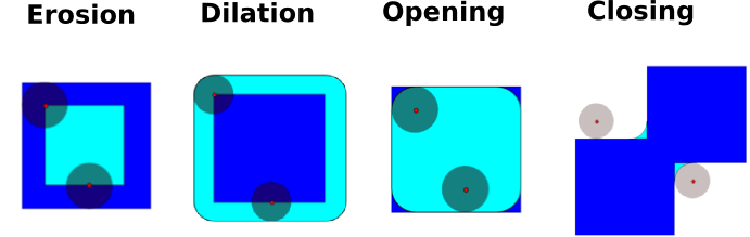
初級數學形態學操作使用結構化的元素,以便修改其他幾何結構。
首先讓我們生成一個結構化元素。
In?[27]:
```
el = ndimage.generate_binary_structure(2, 1)
el
```
Out[27]:
```
array([[False, True, False],
[ True, True, True],
[False, True, False]], dtype=bool)
```
In?[28]:
```
el.astype(np.int)
```
Out[28]:
```
array([[0, 1, 0],
[1, 1, 1],
[0, 1, 0]])
```
* 腐蝕
In?[29]:
```
a = np.zeros((7,7), dtype=np.int)
a[1:6, 2:5] = 1
a
```
Out[29]:
```
array([[0, 0, 0, 0, 0, 0, 0],
[0, 0, 1, 1, 1, 0, 0],
[0, 0, 1, 1, 1, 0, 0],
[0, 0, 1, 1, 1, 0, 0],
[0, 0, 1, 1, 1, 0, 0],
[0, 0, 1, 1, 1, 0, 0],
[0, 0, 0, 0, 0, 0, 0]])
```
In?[30]:
```
ndimage.binary_erosion(a).astype(a.dtype)
```
Out[30]:
```
array([[0, 0, 0, 0, 0, 0, 0],
[0, 0, 0, 0, 0, 0, 0],
[0, 0, 0, 1, 0, 0, 0],
[0, 0, 0, 1, 0, 0, 0],
[0, 0, 0, 1, 0, 0, 0],
[0, 0, 0, 0, 0, 0, 0],
[0, 0, 0, 0, 0, 0, 0]])
```
In?[31]:
```
#腐蝕移除了比結構小的對象
ndimage.binary_erosion(a, structure=np.ones((5,5))).astype(a.dtype)
```
Out[31]:
```
array([[0, 0, 0, 0, 0, 0, 0],
[0, 0, 0, 0, 0, 0, 0],
[0, 0, 0, 0, 0, 0, 0],
[0, 0, 0, 0, 0, 0, 0],
[0, 0, 0, 0, 0, 0, 0],
[0, 0, 0, 0, 0, 0, 0],
[0, 0, 0, 0, 0, 0, 0]])
```
* 擴張
In?[32]:
```
a = np.zeros((5, 5))
a[2, 2] = 1
a
```
Out[32]:
```
array([[ 0., 0., 0., 0., 0.],
[ 0., 0., 0., 0., 0.],
[ 0., 0., 1., 0., 0.],
[ 0., 0., 0., 0., 0.],
[ 0., 0., 0., 0., 0.]])
```
In?[33]:
```
ndimage.binary_dilation(a).astype(a.dtype)
```
Out[33]:
```
array([[ 0., 0., 0., 0., 0.],
[ 0., 0., 1., 0., 0.],
[ 0., 1., 1., 1., 0.],
[ 0., 0., 1., 0., 0.],
[ 0., 0., 0., 0., 0.]])
```
* 開啟
In?[34]:
```
a = np.zeros((5,5), dtype=np.int)
a[1:4, 1:4] = 1; a[4, 4] = 1
a
```
Out[34]:
```
array([[0, 0, 0, 0, 0],
[0, 1, 1, 1, 0],
[0, 1, 1, 1, 0],
[0, 1, 1, 1, 0],
[0, 0, 0, 0, 1]])
```
In?[35]:
```
# 開啟移除了小對象
ndimage.binary_opening(a, structure=np.ones((3,3))).astype(np.int)
```
Out[35]:
```
array([[0, 0, 0, 0, 0],
[0, 1, 1, 1, 0],
[0, 1, 1, 1, 0],
[0, 1, 1, 1, 0],
[0, 0, 0, 0, 0]])
```
In?[36]:
```
# 開啟也可以平滑拐角
ndimage.binary_opening(a).astype(np.int)
```
Out[36]:
```
array([[0, 0, 0, 0, 0],
[0, 0, 1, 0, 0],
[0, 1, 1, 1, 0],
[0, 0, 1, 0, 0],
[0, 0, 0, 0, 0]])
```
* 閉合: `ndimage.binary_closing`
練習
驗證一下開啟相當于先腐蝕再擴張。
開啟操作移除小的結構,而關閉操作填滿了小洞。因此這些用來”清洗“圖像。
In?[37]:
```
a = np.zeros((50, 50))
a[10:-10, 10:-10] = 1
a += 0.25*np.random.standard_normal(a.shape)
mask = a>=0.5
opened_mask = ndimage.binary_opening(mask)
closed_mask = ndimage.binary_closing(opened_mask)
```

練習
驗證一下重建的方格面積比原始方格的面積小。(如果關閉步驟在開啟步驟之前則相反)。
對于_灰度值圖像_,腐蝕(區別于擴張)相當于用感興趣的像素周圍的結構元素中的最小(區別于最大)值替換像素。
In?[39]:
```
a = np.zeros((7,7), dtype=np.int)
a[1:6, 1:6] = 3
a[4,4] = 2; a[2,3] = 1
a
```
Out[39]:
```
array([[0, 0, 0, 0, 0, 0, 0],
[0, 3, 3, 3, 3, 3, 0],
[0, 3, 3, 1, 3, 3, 0],
[0, 3, 3, 3, 3, 3, 0],
[0, 3, 3, 3, 2, 3, 0],
[0, 3, 3, 3, 3, 3, 0],
[0, 0, 0, 0, 0, 0, 0]])
```
In?[40]:
```
ndimage.grey_erosion(a, size=(3,3))
```
Out[40]:
```
array([[0, 0, 0, 0, 0, 0, 0],
[0, 0, 0, 0, 0, 0, 0],
[0, 0, 1, 1, 1, 0, 0],
[0, 0, 1, 1, 1, 0, 0],
[0, 0, 3, 2, 2, 0, 0],
[0, 0, 0, 0, 0, 0, 0],
[0, 0, 0, 0, 0, 0, 0]])
```
### 1.5.10.4 測量圖像
首先讓我們生成一個漂亮的人造二維圖。
In?[41]:
```
x, y = np.indices((100, 100))
sig = np.sin(2*np.pi*x/50.)*np.sin(2*np.pi*y/50.)*(1+x*y/50.**2)**2
mask = sig > 1
```
現在讓我們看一下圖像中對象的各種信息:
In?[42]:
```
labels, nb = ndimage.label(mask)
nb
```
Out[42]:
```
8
```
In?[43]:
```
areas = ndimage.sum(mask, labels, xrange(1, labels.max()+1))
areas
```
Out[43]:
```
array([ 190., 45., 424., 278., 459., 190., 549., 424.])
```
In?[44]:
```
maxima = ndimage.maximum(sig, labels, xrange(1, labels.max()+1))
maxima
```
Out[44]:
```
array([ 1.80238238, 1.13527605, 5.51954079, 2.49611818,
6.71673619, 1.80238238, 16.76547217, 5.51954079])
```
In?[45]:
```
ndimage.find_objects(labels==4)
```
Out[45]:
```
[(slice(30L, 48L, None), slice(30L, 48L, None))]
```
In?[46]:
```
sl = ndimage.find_objects(labels==4)
import pylab as pl
pl.imshow(sig[sl[0]])
```
Out[46]:
```
<matplotlib.image.AxesImage at 0x10a861910>
```


高級例子請看一下總結練習[圖像處理應用:計數氣泡和未融化的顆粒](http://scipy-lectures.github.io/intro/summary-exercises/image-processing.html#summary-exercise-image-processing)
## 1.5.11 科學計算的總結練習
總結練習主要使用Numpy、Scipy 和 Matplotlib。他們提供了一些使用Python進行科學計算的真實例子。現在,已經介紹了Numpy和Scipy的基本使用,邀請感興趣的用戶去做這些練習。
**練習:**
[1.5.11.13 Sprog?氣象站的最大風速預測](http://scipy-lectures.github.io/intro/summary-exercises/stats-interpolate.html)
[1.5.11.14 非線性最小二乘曲線擬合:地形機載激光雷達數據中的點抽取](http://scipy-lectures.github.io/intro/summary-exercises/optimize-fit.html)
[1.5.11.15 圖像處理應用:計數氣泡和未融化的顆粒](http://scipy-lectures.github.io/intro/summary-exercises/image-processing.html)
**提議的解決方案:**
[1.5.11.16 圖像處理練習:玻璃中的未融化顆粒的答案例子](http://scipy-lectures.github.io/intro/summary-exercises/answers_image_processing.html)
### 1.5.11.13 Sprog?氣象站的最大風速預測
這個練習的目的是預測每50年的最大風速,即使在一個時間段內有記錄。可用的數據只是位于丹麥的Sprog?氣象站的21年的測量數據。首先,將給出統計步驟,接著將用scipy.interpolae模塊中的函數來解釋。在最后,將邀請感興趣的讀者用不同的方法從原始數據計算結果。
#### 1.5.11.13.1 統計方法
假設年度最大值符合正態概率密度函數。但是,這個函數不能用來預測,因為它從速度最大值中給出了概率。找到每50年的最大風速需要相反的方法,需要從確定的概率中找到結果。這是百分位數函數的作用而這個練習的目的是找到它。在當前的模型中,假設每50年出現的最大風速定義為高于2%百分位數。
根據定義,百分位數函數是累積分布函數的反函數。后者描述了年度最大值的概率分布。在這個練習中,給定年份$i$的累積概率$p_i$被定義為$p_i = i/(N+1)$,其中$N = 21$,測量的年數。因此,計算每個測量過的風速最大值的累積概率是可以行的。從這些實驗點,scipy.interpolate模塊將對擬合百分位數函數非常有用。最后,50年的最大值將從累積概率的2%百分位數中預估出來。
#### 1.5.11.13.2 計算累積概率
計算好的numpy格式的年度風速最大值存儲在[examples/max-speeds.npy](http://scipy-lectures.github.io/_downloads/max-speeds.npy)文件中, 因此,可以用numpy加載:
In?[4]:
```
import numpy as np
max_speeds = np.load('data/max-speeds.npy')
years_nb = max_speeds.shape[0]
```
下面是前面板塊的累積概率定義$p_i$,對應值將為:
In?[5]:
```
cprob = (np.arange(years_nb, dtype=np.float32) + 1)/(years_nb + 1)
```
并且假設他們可以擬合給定的風速:
In?[6]:
```
sorted_max_speeds = np.sort(max_speeds)
```
#### 1.5.11.13.3 用UnivariateSpline預測
在這個部分,百分位數函數將用`UnivariateSpline`類來估計,這個類用點代表樣條。 默認行為是構建一個3度的樣條,不同的點根據他們的可靠性可能有不同的權重。相關的變體還有`InterpolatedUnivariateSpline`和`LSQUnivariateSpline`,差別在于檢查誤差的方式不同。如果需要2D樣條,可以使用`BivariateSpline`家族類。所有這些1D和2D樣條使用FITPACK Fortran 程序,這就是為什么通過`splrep`和`splev`函數來表征和評估樣條的庫更少。同時,不使用FITPACK參數的插值函數也提供更簡便的用法(見`interp1d`, `interp2d`, `barycentric_interpolate`等等)。 對于Sprog?最大風速的例子,將使用`UnivariateSpline`,因為3度的樣條似乎可以正確擬合數據:
In?[7]:
```
from scipy.interpolate import UnivariateSpline
quantile_func = UnivariateSpline(cprob, sorted_max_speeds)
```
百分位數函數將用評估來所有范圍的概率:
In?[8]:
```
nprob = np.linspace(0, 1, 1e2)
fitted_max_speeds = quantile_func(nprob)
```
在當前的模型中,每50年出現的最大風速被定義為大于2%百分位數。作為結果,累積概率值將是:
In?[9]:
```
fifty_prob = 1. - 0.02
```
因此,可以猜測50年一遇的暴風雪風速為:
In?[10]:
```
fifty_wind = quantile_func(fifty_prob)
fifty_wind
```
Out[10]:
```
array(32.97989825386221)
```
現在,結果被收集在Matplotlib圖片中:

答案:[Python源文件](http://scipy-lectures.github.io/intro/summary-exercises/auto_examples/plot_cumulative_wind_speed_prediction.html#example-plot-cumulative-wind-speed-prediction-py)
#### 1.5.11.13.4 Gumbell分布練習
現在邀請感興趣的讀者用21年測量的風速做一個練習。測量區間為90分鐘(原始的區間約為10分鐘,但是,為了讓練習的設置簡單一些,縮小了文件的大小)。數據以numpy格式存儲在文件[examples/sprog-windspeeds.npy](http://scipy-lectures.github.io/_downloads/sprog-windspeeds.npy)中。 在完成練習后,不要看繪圖的源代碼。
* 第一步將是通過使用numpy來找到年度最大值,然后將它們繪制為matplotlibe條形圖。 
答案:[Python源文件](http://scipy-lectures.github.io/intro/summary-exercises/auto_examples/plot_sprog_annual_maxima.html#example-plot-sprog-annual-maxima-py)
* 第二步將是在累積概率$p_i$使用Gumbell分布,$p_i$的定義是$-log( -log(p_i) )$用來擬合線性百分位數函數(記住你可以定義UnivariateSpline的度數)。 繪制年度最大值和Gumbell分布將生產如下圖片。

答案:[Python源文件](http://scipy-lectures.github.io/intro/summary-exercises/auto_examples/plot_gumbell_wind_speed_prediction.html#example-plot-gumbell-wind-speed-prediction-py)
* 最后一步將是找到在每50年出現的最大風速34.23 m/s。
### 1.5.11.14 非線性最小二乘曲線擬合:地理雷達數據中的點抽取應用
這個練習的目的是用模型去擬合一些數據。這篇教程中的數據是雷達數據,下面的介紹段落將詳細介紹。如果你沒有耐心,想要馬上進行聯系,那么請跳過這部分,并直接進入[加載和可視化](http://scipy-lectures.github.io/intro/summary-exercises/optimize-fit.html#first-step)。
#### 1.5.11.14.1 介紹
雷達系統是光學測距儀,通過分析離散光的屬性來測量距離。絕大多數光學測距儀向目標發射一段短光學脈沖,然后記錄反射信號。然后處理這個信號來抽取雷達系統與目標間的距離。
地形雷達系統是嵌入在飛行平臺的雷達系統。它們測量平臺與地球的距離,以便計算出地球的地形信息(更多細節見[[1]](http://scipy-lectures.github.io/intro/summary-exercises/optimize-fit.html#mallet))。
[1] Mallet, C. and Bretar, F. Full-Waveform Topographic Lidar: State-of-the-Art. ISPRS Journal of Photogrammetry and Remote Sensing 64(1), pp.1-16, January 2009 [http://dx.doi.org/10.1016/j.isprsjprs.2008.09.007](http://dx.doi.org/10.1016/j.isprsjprs.2008.09.007)
這篇教程的目的是分析雷達系統記錄到的波形數據[[2]](http://scipy-lectures.github.io/intro/summary-exercises/optimize-fit.html#data)。這種信號包含波峰,波峰的中心和振幅可以用來計算命中目標的位置和一些特性。當激光柱的腳步距離地球表面1m左右,光柱可以在二次傳播時擊中多個目標(例如,地面和樹木或建筑的頂部)。激光柱的擊中每個目標的貢獻之和會產生一個有多個波峰的復雜波,每一個包含一個目標的信息。
一種從這些數據中抽取信息的先進方法是在一個高斯函數和中分解這些信息,每個函數代表激光柱擊中的一個目標的貢獻。
因此,我們使用`the scipy.optimize`模塊將波形擬合為一個高斯函數或高斯函數之和。
#### 1.5.11.14.2 加載和可視化
加載第一個波形:
In?[1]:
```
import numpy as np
waveform_1 = np.load('data/waveform_1.npy')
```
接著可視化:
In?[2]:
```
import matplotlib.pyplot as plt
t = np.arange(len(waveform_1))
plt.plot(t, waveform_1)
plt.show()
```

你可以注意到,這個波形是單峰80個區間的信息。
#### 1.5.11.14.3 用簡單的高斯模型擬合波形
這個信號非常簡單,可以被建模為一個高斯函數,抵消相應的背景噪音。要用函數擬合這個信號,我們必須:
* 定義一個模型
* 給出初始解
* 調用`scipy.optimize.leastsq`
##### 1.5.11.14.3.1 模型
高斯函數定義如下:
$B + A \exp\left\{-\left(\frac{t-\mu}{\sigma}\right)^2\right\}$
在Python中定義如下:
In?[3]:
```
def model(t, coeffs):
return coeffs[0] + coeffs[1] * np.exp( - ((t-coeffs[2])/coeffs[3])**2 )
```
其中
* coeffs[0] is $B$ (noise)
* coeffs[1] is $A$ (amplitude)
* coeffs[2] is $\mu$ (center)
* coeffs[3] is $\sigma$ (width)
##### 1.5.11.14.3.2 初始解
通過觀察圖形,我們可以找到大概的初始解,例如:
In?[5]:
```
x0 = np.array([3, 30, 15, 1], dtype=float)
```
##### 1.5.11.14.3.3 擬合
`scipy.optimize.leastsq`最小化作為參數給到的函數的平方和。本質上來說,函數最小化的是殘差(數據與模型的差異):
In?[6]:
```
def residuals(coeffs, y, t):
return y - model(t, coeffs)
```
因此,讓我們通過下列參數調用`scipy.optimize.leastsq`來求解:
* 最小化的函數
* 初始解
* 傳遞給函數的額外參數
In?[7]:
```
from scipy.optimize import leastsq
x, flag = leastsq(residuals, x0, args=(waveform_1, t))
print x
```
```
[ 2.70363341 27.82020741 15.47924562 3.05636228]
```
答案可視化:
In?[8]:
```
plt.plot(t, waveform_1, t, model(t, x))
plt.legend(['waveform', 'model'])
plt.show()
```

備注:從scipy v0.8及以上,你應該使用`scipy.optimize.curve_fit`,它使用模型和數據作為參數,因此,你不再需要定義殘差。
#### 1.5.11.14.4 更進一步
* 試一下包含三個波峰的更復雜波形(例如[data/waveform_2.npy](https://github.com/scipy-lectures/scipy-lecture-notes/raw/master/data/waveform_2.npy))。你必須調整模型,現在它是高斯函數之和,而不是只有一個高斯波峰。

* 在一些情況下,寫一個函數來計算Jacobian,要比讓leastsq從數值上估計它來的快。創建一個函數來計算殘差的Jacobian,并且用它作為leastsq的一個輸入。
* 當我們想要識別信號中非常小的峰值,或者初始的猜測離好的解決方案太遠時,算法給出的結果往往不能令人滿意。為模型參數添加限制可以確保克服這些局限性。我們可以添加的先前經驗是變量的符號(都是正的)。
用下列初始解:
In?[9]:
```
x0 = np.array([3, 50, 20, 1], dtype=float)
```
添加了邊界限制之后比較一下`scipy.optimize.leastsq`與`scipy.optimize.fmin_slsqp`的結果。
[2] 本教程的數據部分來自于[FullAnalyze software](http://fullanalyze.sourceforge.net/)的演示數據,由 [GIS DRAIX](http://www.ore.fr/rubrique.php3?id_rubrique=24) 友情提供。
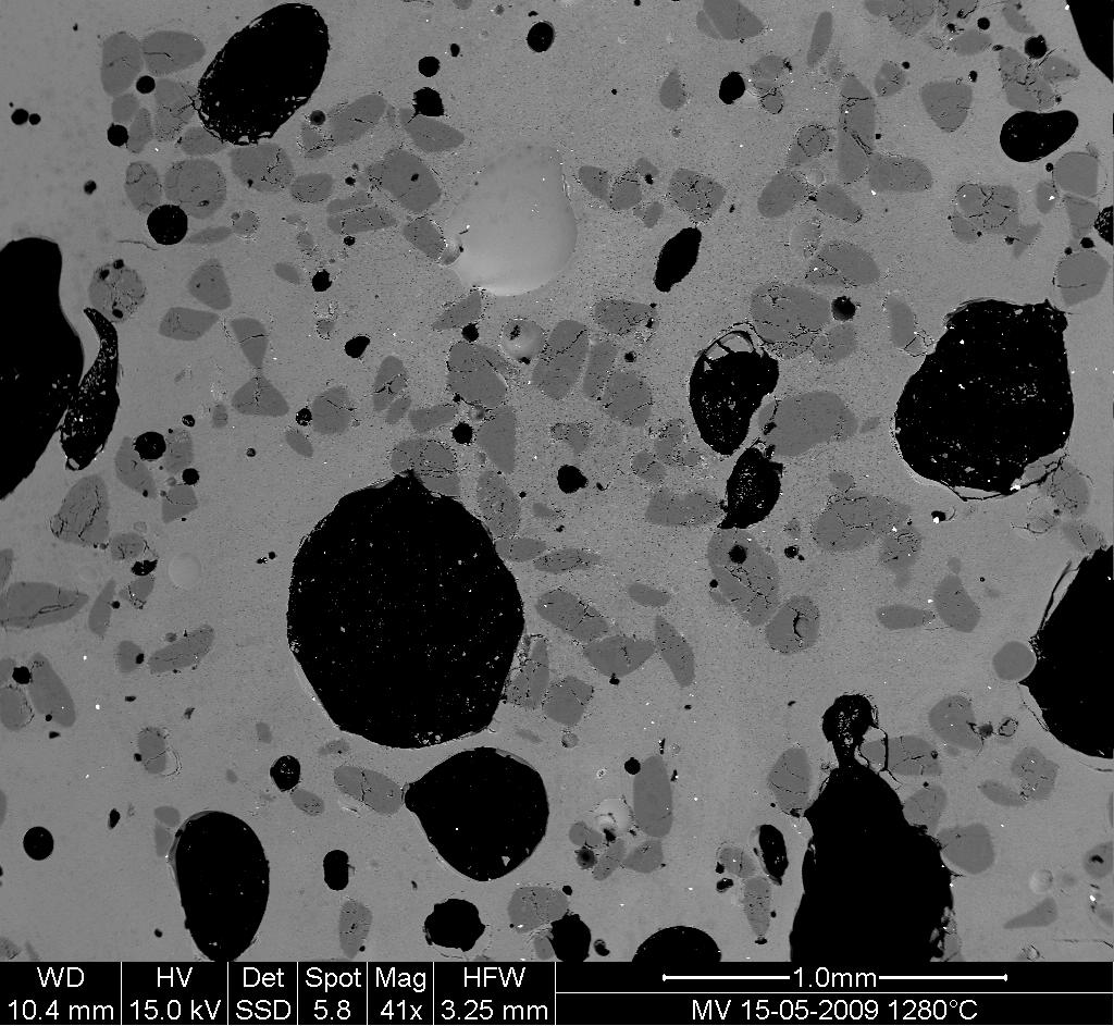
### 1.5.11.15 圖像處理應用:計數氣泡和未融化的顆粒
#### 1.5.11.15.1 問題描述
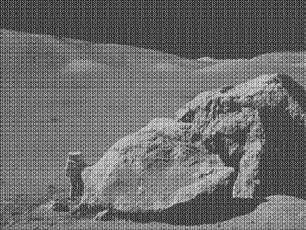
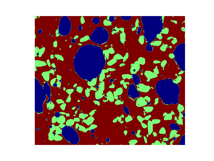
1. 打開圖像文件MV_HFV_012.jpg并且瀏覽一下。看一下imshow文檔字符串中的參數,用“右”對齊來顯示圖片(原點在左下角,而不是像標準數組在右上角)。
這個掃描元素顯微圖顯示了一個帶有一些氣泡(黑色)和未溶解沙(深灰)的玻璃樣本(輕灰矩陣)。我們想要判斷樣本由三個狀態覆蓋的百分比,并且預測沙粒和氣泡的典型大小和他們的大小等。
2. 修建圖片,刪除帶有測量信息中底部面板。
3. 用中位數過濾稍稍過濾一下圖像以便改進它的直方圖。看一下直方圖的變化。
4. 使用過濾后圖像的直方圖,決定允許定義沙粒像素,玻璃像素和氣泡像素掩蔽的閾限。其他的選項(家庭作業):寫一個函數從直方圖的最小值自動判斷閾限。
5. 將三種不同的相用不同的顏色上色并顯示圖片。
6. 用數學形態學清理不同的相。
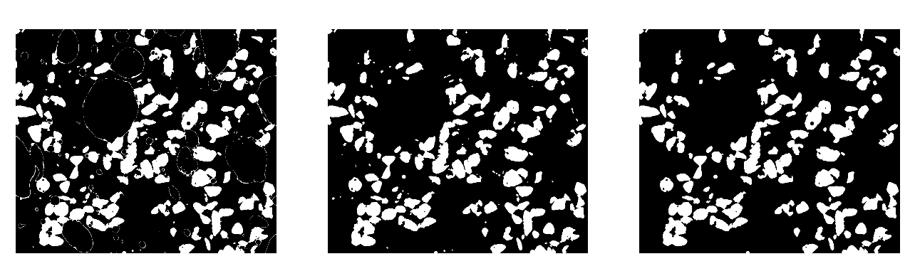
7. 為所有氣泡和沙粒做標簽,從沙粒中刪除小于10像素的掩蔽。要這樣做,用`ndimage.sum`或`np.bincount`來計算沙粒大小。
8. 計算氣泡的平均大小。
### 1.5.11.16 圖像處理練習:玻璃中的未融化顆粒的答案例子
In?[1]:
```
import numpy as np
import pylab as pl
from scipy import ndimage
```

* 打開圖像文件MV_HFV_012.jpg并且瀏覽一下。看一下imshow文檔字符串中的參數,用“右”對齊來顯示圖片(原點在左下角,而不是像標準數組在右上角)。
In?[3]:
```
dat = pl.imread('data/MV_HFV_012.jpg')
```
* 修建圖片,刪除帶有測量信息中底部面板。
In?[4]:
```
dat = dat[60:]
```
* 用中位數過濾稍稍過濾一下圖像以便改進它的直方圖。看一下直方圖的變化。
In?[5]:
```
filtdat = ndimage.median_filter(dat, size=(7,7))
hi_dat = np.histogram(dat, bins=np.arange(256))
hi_filtdat = np.histogram(filtdat, bins=np.arange(256))
```
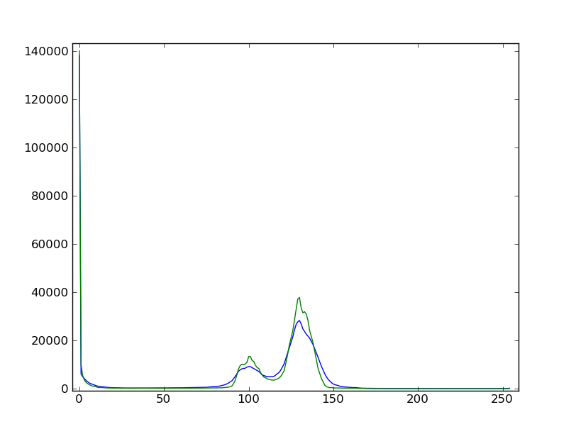
* 使用過濾后圖像的直方圖,決定允許定義沙粒像素,玻璃像素和氣泡像素掩蔽的閾限。其他的選項(家庭作業):寫一個函數從直方圖的最小值自動判斷閾限。
In?[6]:
```
void = filtdat <= 50
sand = np.logical_and(filtdat > 50, filtdat <= 114)
glass = filtdat > 114
```
* 將三種不同的相用不同的顏色上色并顯示圖片。
In?[7]:
```
phases = void.astype(np.int) + 2*glass.astype(np.int) + 3*sand.astype(np.int)
```
* 用數學形態學清理不同的相。
In?[8]:
```
sand_op = ndimage.binary_opening(sand, iterations=2)
```
* 為所有氣泡和沙粒做標簽,從沙粒中刪除小于10像素的掩蔽。要這樣做,用`ndimage.sum`或`np.bincount`來計算沙粒大小。
In?[9]:
```
sand_labels, sand_nb = ndimage.label(sand_op)
sand_areas = np.array(ndimage.sum(sand_op, sand_labels, np.arange(sand_labels.max()+1)))
mask = sand_areas > 100
remove_small_sand = mask[sand_labels.ravel()].reshape(sand_labels.shape)
```
* 計算氣泡的平均大小。
In?[10]:
```
bubbles_labels, bubbles_nb = ndimage.label(void)
bubbles_areas = np.bincount(bubbles_labels.ravel())[1:]
mean_bubble_size = bubbles_areas.mean()
median_bubble_size = np.median(bubbles_areas)
mean_bubble_size, median_bubble_size
```
Out[10]:
```
(2416.863157894737, 60.0)
```
- 介紹
- 1.1 科學計算工具及流程
- 1.2 Python語言
- 1.3 NumPy:創建和操作數值數據
- 1.4 Matplotlib:繪圖
- 1.5 Scipy:高級科學計算
- 1.6 獲取幫助及尋找文檔
- 2.1 Python高級功能(Constructs)
- 2.2 高級Numpy
- 2.3 代碼除錯
- 2.4 代碼優化
- 2.5 SciPy中稀疏矩陣
- 2.6 使用Numpy和Scipy進行圖像操作及處理
- 2.7 數學優化:找到函數的最優解
- 2.8 與C進行交互
- 3.1 Python中的統計學
- 3.2 Sympy:Python中的符號數學
- 3.3 Scikit-image:圖像處理
- 3.4 Traits:創建交互對話
- 3.5 使用Mayavi進行3D作圖
- 3.6 scikit-learn:Python中的機器學習