2.6 使用Numpy和Scipy進行圖像操作及處理 · SciPy Lecture Notes 中文版

# 2.6 使用Numpy和Scipy進行圖像操作及處理 In?[3]: ``` %matplotlib inline import numpy as np ``` **作者**：Emmanuelle Gouillart, Ga?l Varoquaux 這個部分解決用核心的科學模塊NumPy和SciPy做基本的圖像操作和處理。這個教程中涵蓋的一些操作可能對于一些其他類型的多維度數據處理比對圖像處理更加有用。特別是，子摸塊[scipy.ndimage](http://docs.scipy.org/doc/scipy/reference/ndimage.html#module-scipy.ndimage)提供了在N維Numpy數組上操作的方法。 **也看一下:** 對于更高級的圖像處理和圖像特有的程序，見專注于[skimage](http://scikit-image.org/docs/stable/api/skimage.html#module-skimage)模塊教程[Scikit-image: 圖像處理](http://www.scipy-lectures.org/packages/scikit-image/index.html#scikit-image)。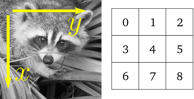 **圖像 = 2-D 數值數組** (或者 3-D: CT, MRI, 2D + time; 4-D, ...) 這里, **圖像 == Numpy 數組** `np.array` **本教程中使用的工具:** * `numpy`: 基礎的數組操作 * `scipy`: `scipy.ndimage` 專注于圖像處理的子模塊 (n維圖像)。見[文檔](http://docs.scipy.org/doc/scipy/reference/tutorial/ndimage.html): In?[1]: ``` from scipy import ndimage ``` **圖像處理中的常見任務:** * 輸入/輸出、顯示圖像 * 基礎操作: 剪切, 翻轉、旋轉... * 圖像過濾: 降噪, 銳化 * 圖形分割: 根據不同的對象標記像素 * 分類 * 特征提取 * 配準 * ... **章節內容** ``` 打開和寫入圖像文件顯示圖像基礎操作統計信息幾何圖像變換圖像過濾模糊/光滑銳化降噪數學形態學特征提取邊緣檢測分隔測量對象屬性: ndimage.measurements ``` ## 2.6.1 打開和寫入圖像文件將數組寫入文件: In?[4]: ``` from scipy import misc f = misc.face() misc.imsave('face.png', f) # 使用圖像模塊 (PIL) import matplotlib.pyplot as plt plt.imshow(f) plt.show() ``` ![](https://box.kancloud.cn/2016-03-21_56efdc0a82128.png) 從圖像文件創建一個numpy數組: In?[5]: ``` from scipy import misc face = misc.face() misc.imsave('face.png', face) # 首先我們需要創建這個PNG文件 face = misc.imread('face.png') type(face) ``` Out[5]: ``` numpy.ndarray ``` In?[6]: ``` face.shape, face.dtype ``` Out[6]: ``` ((768, 1024, 3), dtype('uint8')) ``` 對于8位的圖像 (0-255) dtype是uint8 打開raw文件 (照相機, 3-D 圖像) In?[7]: ``` face.tofile('face.raw') # 創建raw文件 face_from_raw = np.fromfile('face.raw', dtype=np.uint8) face_from_raw.shape ``` Out[7]: ``` (2359296,) ``` In?[8]: ``` face_from_raw.shape = (768, 1024, 3) ``` 需要知道圖像的shape和dtype (如何去分離數據類型)。對于大數據, 使用`np.memmap`來做內存映射: In?[9]: ``` face_memmap = np.memmap('face.raw', dtype=np.uint8, shape=(768, 1024, 3)) ``` (數據從文件中讀取，并沒有加載到內存) 處理一組圖像文件 In?[10]: ``` for i in range(10): im = np.random.random_integers(0, 255, 10000).reshape((100, 100)) misc.imsave('random_%02d.png' % i, im) from glob import glob filelist = glob('random*.png') filelist.sort() ``` ## 2.6.2 顯示圖像使用`matplotlib`和`imshow`在`matplotlib圖形內部`顯示圖像: In?[11]: ``` f = misc.face(gray=True) # 取回灰度圖像 import matplotlib.pyplot as plt plt.imshow(f, cmap=plt.cm.gray) ``` Out[11]: ``` <matplotlib.image.AxesImage at 0x10afb0bd0> ``` ![](https://box.kancloud.cn/2016-03-21_56efdc0aa0095.png) 通過設置最小和最大值增加對比度: In?[14]: ``` plt.imshow(f, cmap=plt.cm.gray, vmin=30, vmax=200) ``` Out[14]: ``` <matplotlib.image.AxesImage at 0x110f8c6d0> ``` ![](https://box.kancloud.cn/2016-03-21_56efdc0ac9b02.png) In?[16]: ``` plt.imshow(f, cmap=plt.cm.gray, vmin=30, vmax=200) # 刪除座標軸和刻度 plt.axis('off') ``` Out[16]: ``` (-0.5, 1023.5, 767.5, -0.5) ``` ![](https://box.kancloud.cn/2016-03-21_56efdc0aeef69.png) 畫出輪廓線: In?[18]: ``` plt.imshow(f, cmap=plt.cm.gray, vmin=30, vmax=200) # 刪除座標軸和刻度 plt.axis('off') plt.contour(f, [50, 200]) ``` Out[18]: ``` <matplotlib.contour.QuadContourSet instance at 0x10cab5878> ``` ![](https://box.kancloud.cn/2016-03-21_56efdc0b1d597.png) [[Python 源代碼]](http://www.scipy-lectures.org/advanced/image_processing/auto_examples/plot_display_face.html#example-plot-display-face-py) 對于要精確檢查的密度變量，使用`interpolation='nearest'`: In?[19]: ``` plt.imshow(f[320:340, 510:530], cmap=plt.cm.gray) ``` Out[19]: ``` <matplotlib.image.AxesImage at 0x10590da90> ``` ![](https://box.kancloud.cn/2016-03-21_56efdc0b3d633.png) In?[20]: ``` plt.imshow(f[320:340, 510:530], cmap=plt.cm.gray, interpolation='nearest') ``` Out[20]: ``` <matplotlib.image.AxesImage at 0x110716c10> ``` ![](https://box.kancloud.cn/2016-03-21_56efdc0b54207.png) [[Python 源代碼]](http://www.scipy-lectures.org/advanced/image_processing/auto_examples/plot_interpolation_face.html#example-plot-interpolation-face-py) **也可以看一下** 3-D 可視化: Mayavi 見[使用Mayavi的3D繪圖](http://www.scipy-lectures.org/packages/3d_plotting/index.html#mayavi-label)。 * Image plane widgets * Isosurfaces * ... ![](http://www.scipy-lectures.org/_images/decorations.png) ## 2.6.3 基礎操作圖像是數組: 使用完整的numpy機制。 ![](http://www.scipy-lectures.org/_images/axis_convention.png) In?[21]: ``` face = misc.face(gray=True) face[0, 40] ``` Out[21]: ``` 127 ``` In?[22]: ``` # 切片 face[10:13, 20:23] ``` Out[22]: ``` array([[141, 153, 145], [133, 134, 125], [ 96, 92, 94]], dtype=uint8) ``` In?[24]: ``` face[100:120] = 255 lx, ly = face.shape X, Y = np.ogrid[0:lx, 0:ly] mask = (X - lx / 2) ** 2 + (Y - ly / 2) ** 2 > lx * ly / 4 # 掩碼（masks） face[mask] = 0 # 象征索引（Fancy indexing） face[range(400), range(400)] = 255 ``` ![](http://www.scipy-lectures.org/_images/plot_numpy_array_1.png) [[Python source code]](http://www.scipy-lectures.org/advanced/image_processing/auto_examples/plot_numpy_array.html#example-plot-numpy-array-py) ### 2.6.3.1 統計信息 In?[26]: ``` face = misc.face(gray=True) face.mean() ``` Out[26]: ``` 113.48026784261067 ``` In?[27]: ``` face.max(), face.min() ``` Out[27]: ``` (250, 0) ``` `np.histogram` **練習** * 將`scikit-image` logo作為數組打開 ([http://scikit-image.org/_static/img/logo.png](http://scikit-image.org/_static/img/logo.png)), 或者在你電腦上的其他圖像。 * 剪切圖像的有意義部分，例如，logo中的python圓形。 * 用`matplotlib`顯示圖像數組。改變interpolation方法并且放大看一下差異。 * 將你的圖像改變為灰度 * 通過改變它的最小最大值增加圖像的對比度。**選做：**使用`scipy.stats.scoreatpercentile` (讀一下文本字符串!) 來飽和最黑5%的像素和最亮5%的像素。 * 將數組保存為兩個不同的文件格式 (png, jpg, tiff) ![](http://www.scipy-lectures.org/_images/scikit_image_logo.png) ### 2.6.3.2 幾何圖像變換 In?[28]: ``` face = misc.face(gray=True) lx, ly = face.shape # 剪切 crop_face = face[lx / 4: - lx / 4, ly / 4: - ly / 4] # up <-> down 翻轉 flip_ud_face = np.flipud(face) # 旋轉 rotate_face = ndimage.rotate(face, 45) rotate_face_noreshape = ndimage.rotate(face, 45, reshape=False) ``` ![](http://www.scipy-lectures.org/_images/plot_geom_face_1.png) [[Python source code]](http://www.scipy-lectures.org/advanced/image_processing/auto_examples/plot_geom_face.html#example-plot-geom-face-py) ## 2.6.4 圖像過濾 **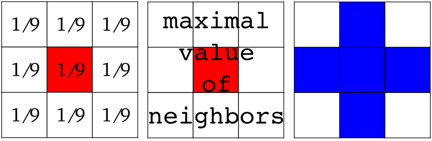局部過濾器**: 通過臨近像素值的函數來替換像素的值。 **鄰居**: 方塊 (選擇大小)、硬盤、或者更復雜的結構化元素。 ![](http://www.scipy-lectures.org/_images/kernels.png) ### 2.6.4.1 模糊 / 光滑 **高斯過濾器** 來自 `scipy.ndimage`: In?[29]: ``` from scipy import misc face = misc.face(gray=True) blurred_face = ndimage.gaussian_filter(face, sigma=3) very_blurred = ndimage.gaussian_filter(face, sigma=5) ``` **均勻過濾器** In?[30]: ``` local_mean = ndimage.uniform_filter(face, size=11) ``` ![](http://www.scipy-lectures.org/_images/plot_blur_1.png) [[Python source code]](http://www.scipy-lectures.org/advanced/image_processing/auto_examples/plot_blur.html) ### 2.6.4.2 銳化銳化模糊的圖像: In?[31]: ``` from scipy import misc face = misc.face(gray=True).astype(float) blurred_f = ndimage.gaussian_filter(face, 3) ``` 通過添加Laplacian的近似值來增加邊緣的權重: In?[32]: ``` filter_blurred_f = ndimage.gaussian_filter(blurred_f, 1) alpha = 30 sharpened = blurred_f + alpha * (blurred_f - filter_blurred_f) ``` ![](http://www.scipy-lectures.org/_images/plot_sharpen_1.png) [[Python source code]](http://www.scipy-lectures.org/advanced/image_processing/auto_examples/plot_sharpen.html#example-plot-sharpen-py) ### 2.6.4.3 降噪有噪音的臉: In?[33]: ``` from scipy import misc f = misc.face(gray=True) f = f[230:290, 220:320] noisy = f + 0.4 * f.std() * np.random.random(f.shape) ``` **高斯過濾器**光滑了噪音... 以及邊緣: In?[34]: ``` gauss_denoised = ndimage.gaussian_filter(noisy, 2) ``` 絕大多數局部線性各向同性過濾器模糊圖像 (`ndimage.uniform_filter`) **中位數過濾器**更好的保留的邊緣: In?[35]: ``` med_denoised = ndimage.median_filter(noisy, 3) ``` ![](http://www.scipy-lectures.org/_images/plot_face_denoise_1.png) [[Python source code]](http://www.scipy-lectures.org/advanced/image_processing/auto_examples/plot_face_denoise.html#example-plot-face-denoise-py) 中位數過濾器: 對直邊緣的結果更好 (低曲度): In?[37]: ``` im = np.zeros((20, 20)) im[5:-5, 5:-5] = 1 im = ndimage.distance_transform_bf(im) im_noise = im + 0.2 * np.random.randn(*im.shape) im_med = ndimage.median_filter(im_noise, 3) ``` ![](http://www.scipy-lectures.org/_images/plot_denoising_1.png) [[Python source code]](http://www.scipy-lectures.org/advanced/image_processing/auto_examples/plot_denoising.html) 其他排名過濾器：`ndimage.maximum_filter`、`ndimage.percentile_filter` 其他的局部非線性過濾器: Wiener (`scipy.signal.wiener`) 等等. **非局部過濾器** **練習: 降噪** * 創建一個帶有一些對象 (圓形、橢圓、正方形或隨機形狀) 的二元圖像 (0 和 1) . * 添加一些噪音 (例如, 20% 的噪音) * 用兩種不同的降噪方法來降噪這個圖像: 高斯過濾器和中位數過濾器。 * 比較兩種不同降噪方法的直方圖。哪一個與原始圖像（無噪音）的直方圖最接近? **也看一下：** 在`skimage.denoising`中有更多的的降噪過濾器可用，見教程[Scikit-image: 圖像處理](http://www.scipy-lectures.org/packages/scikit-image/index.html#scikit-image). ### 2.6.4.4 數學形態學看一下[wikipedia](https://en.wikipedia.org/wiki/Mathematical_morphology)上的數學形態學定義。探索一個簡單形狀 (結構化的元素) 的圖像，然后根據這個形狀是如何局部適應或不適應這個圖像來修改這個圖像。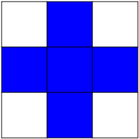 **結構化元素:** In?[38]: ``` el = ndimage.generate_binary_structure(2, 1) el ``` Out[38]: ``` array([[False, True, False], [ True, True, True], [False, True, False]], dtype=bool) ``` In?[39]: ``` el.astype(np.int) ``` Out[39]: ``` array([[0, 1, 0], [1, 1, 1], [0, 1, 0]]) ``` ![](http://www.scipy-lectures.org/_images/diamond_kernel.png) **風化(Erosion)** = 最小值過濾器。用結構化元素所覆蓋的最小值來替換像素的值。: In?[41]: ``` a = np.zeros((7,7), dtype=np.int) a[1:6, 2:5] = 1 a ``` Out[41]: ``` array([[0, 0, 0, 0, 0, 0, 0], [0, 0, 1, 1, 1, 0, 0], [0, 0, 1, 1, 1, 0, 0], [0, 0, 1, 1, 1, 0, 0], [0, 0, 1, 1, 1, 0, 0], [0, 0, 1, 1, 1, 0, 0], [0, 0, 0, 0, 0, 0, 0]]) ``` In?[42]: ``` ndimage.binary_erosion(a).astype(a.dtype) ``` Out[42]: ``` array([[0, 0, 0, 0, 0, 0, 0], [0, 0, 0, 0, 0, 0, 0], [0, 0, 0, 1, 0, 0, 0], [0, 0, 0, 1, 0, 0, 0], [0, 0, 0, 1, 0, 0, 0], [0, 0, 0, 0, 0, 0, 0], [0, 0, 0, 0, 0, 0, 0]]) ``` In?[43]: ``` #風化刪除了比結構小的對象 ndimage.binary_erosion(a, structure=np.ones((5,5))).astype(a.dtype) ``` Out[43]: ``` array([[0, 0, 0, 0, 0, 0, 0], [0, 0, 0, 0, 0, 0, 0], [0, 0, 0, 0, 0, 0, 0], [0, 0, 0, 0, 0, 0, 0], [0, 0, 0, 0, 0, 0, 0], [0, 0, 0, 0, 0, 0, 0], [0, 0, 0, 0, 0, 0, 0]]) ``` ![](http://www.scipy-lectures.org/_images/morpho_mat.png) **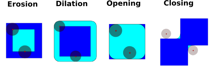擴大(Dilation)**：最大值過濾器： In?[44]: ``` a = np.zeros((5, 5)) a[2, 2] = 1 a ``` Out[44]: ``` array([[ 0., 0., 0., 0., 0.], [ 0., 0., 0., 0., 0.], [ 0., 0., 1., 0., 0.], [ 0., 0., 0., 0., 0.], [ 0., 0., 0., 0., 0.]]) ``` In?[45]: ``` ndimage.binary_dilation(a).astype(a.dtype) ``` Out[45]: ``` array([[ 0., 0., 0., 0., 0.], [ 0., 0., 1., 0., 0.], [ 0., 1., 1., 1., 0.], [ 0., 0., 1., 0., 0.], [ 0., 0., 0., 0., 0.]]) ``` 對于灰度值圖像同樣適用: In?[46]: ``` np.random.seed(2) im = np.zeros((64, 64)) x, y = (63*np.random.random((2, 8))).astype(np.int) im[x, y] = np.arange(8) bigger_points = ndimage.grey_dilation(im, size=(5, 5), structure=np.ones((5, 5))) square = np.zeros((16, 16)) square[4:-4, 4:-4] = 1 dist = ndimage.distance_transform_bf(square) dilate_dist = ndimage.grey_dilation(dist, size=(3, 3), structure=np.ones((3, 3))) ``` ![](http://www.scipy-lectures.org/_images/plot_greyscale_dilation_1.png) [[Python source code]](http://www.scipy-lectures.org/advanced/image_processing/auto_examples/plot_greyscale_dilation.html) **Opening**: erosion + dilation: In?[48]: ``` a = np.zeros((5,5), dtype=np.int) a[1:4, 1:4] = 1; a[4, 4] = 1 a ``` Out[48]: ``` array([[0, 0, 0, 0, 0], [0, 1, 1, 1, 0], [0, 1, 1, 1, 0], [0, 1, 1, 1, 0], [0, 0, 0, 0, 1]]) ``` In?[49]: ``` # Opening 刪除小對象 ndimage.binary_opening(a, structure=np.ones((3,3))).astype(np.int) ``` Out[49]: ``` array([[0, 0, 0, 0, 0], [0, 1, 1, 1, 0], [0, 1, 1, 1, 0], [0, 1, 1, 1, 0], [0, 0, 0, 0, 0]]) ``` In?[50]: ``` # Opening 也可以光滑轉角 ndimage.binary_opening(a).astype(np.int) ``` Out[50]: ``` array([[0, 0, 0, 0, 0], [0, 0, 1, 0, 0], [0, 1, 1, 1, 0], [0, 0, 1, 0, 0], [0, 0, 0, 0, 0]]) ``` **應用**: 去除噪音: In?[51]: ``` square = np.zeros((32, 32)) square[10:-10, 10:-10] = 1 np.random.seed(2) x, y = (32*np.random.random((2, 20))).astype(np.int) square[x, y] = 1 open_square = ndimage.binary_opening(square) eroded_square = ndimage.binary_erosion(square) reconstruction = ndimage.binary_propagation(eroded_square, mask=square) ``` ![](http://www.scipy-lectures.org/_images/plot_propagation_1.png) [[Python source code]](http://www.scipy-lectures.org/advanced/image_processing/auto_examples/plot_propagation.html) **Closing**: dilation + erosion 許多其他的數學形態學操作: hit 和 miss 轉換、tophat等等。 ### 2.6.5.2 分割 * 直方圖分割 (沒有空間信息) In?[52]: ``` n = 10 l = 256 im = np.zeros((l, l)) np.random.seed(1) points = l*np.random.random((2, n**2)) im[(points[0]).astype(np.int), (points[1]).astype(np.int)] = 1 im = ndimage.gaussian_filter(im, sigma=l/(4.*n)) mask = (im > im.mean()).astype(np.float) mask += 0.1 * im img = mask + 0.2*np.random.randn(*mask.shape) hist, bin_edges = np.histogram(img, bins=60) bin_centers = 0.5*(bin_edges[:-1] + bin_edges[1:]) binary_img = img > 0.5 ``` ![](http://www.scipy-lectures.org/_images/plot_histo_segmentation_1.png) [[Python source code]](http://www.scipy-lectures.org/advanced/image_processing/auto_examples/plot_histo_segmentation.html) 用數學形態學來清理結果: In?[53]: ``` # 刪除小白色區域 open_img = ndimage.binary_opening(binary_img) # 刪除小黑洞 close_img = ndimage.binary_closing(open_img) ``` ![](http://www.scipy-lectures.org/_images/plot_clean_morpho_1.png) [[Python source code]](http://www.scipy-lectures.org/advanced/image_processing/auto_examples/plot_clean_morpho.html) **練習** 檢查重建操作 (erosion + propagation) 生成一個比opening/closing更好的結果: In?[55]: ``` eroded_img = ndimage.binary_erosion(binary_img) reconstruct_img = ndimage.binary_propagation(eroded_img, mask=binary_img) tmp = np.logical_not(reconstruct_img) eroded_tmp = ndimage.binary_erosion(tmp) reconstruct_final = np.logical_not(ndimage.binary_propagation(eroded_tmp, mask=tmp)) np.abs(mask - close_img).mean() ``` Out[55]: ``` 0.0072783654884356133 ``` In?[56]: ``` np.abs(mask - reconstruct_final).mean() ``` Out[56]: ``` 0.00059502552803868841 ``` **練習** 檢查第一步降噪 (例如，中位數過濾器) 如何影響直方圖，檢查產生的基于直方圖的分割是否更加準確。 **也可以看一下**：更高級分割算法可以在`scikit-image`中找到: 見[Scikit-image: 圖像處理](http://www.scipy-lectures.org/packages/scikit-image/index.html#scikit-image)。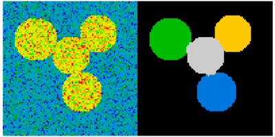 **也可以看一下**：其他科學計算包為圖像處理提供的算法。在這個例子中，我們使用`scikit-learn`中的譜聚類函數以便分割黏在一起的對象。 In?[57]: ``` from sklearn.feature_extraction import image from sklearn.cluster import spectral_clustering l = 100 x, y = np.indices((l, l)) center1 = (28, 24) center2 = (40, 50) center3 = (67, 58) center4 = (24, 70) radius1, radius2, radius3, radius4 = 16, 14, 15, 14 circle1 = (x - center1[0])**2 + (y - center1[1])**2 < radius1**2 circle2 = (x - center2[0])**2 + (y - center2[1])**2 < radius2**2 circle3 = (x - center3[0])**2 + (y - center3[1])**2 < radius3**2 circle4 = (x - center4[0])**2 + (y - center4[1])**2 < radius4**2 # 4個圓形 img = circle1 + circle2 + circle3 + circle4 mask = img.astype(bool) img = img.astype(float) img += 1 + 0.2*np.random.randn(*img.shape) # 將圖像轉化為邊緣帶有坡度值的圖。 graph = image.img_to_graph(img, mask=mask) # 用一個梯度遞減函數: 我們用它輕度依賴于接近voronoi的梯度細分 graph.data = np.exp(-graph.data/graph.data.std()) labels = spectral_clustering(graph, n_clusters=4, eigen_solver='arpack') label_im = -np.ones(mask.shape) label_im[mask] = labels ``` ![](http://www.scipy-lectures.org/_images/image_spectral_clustering.png) ## 2.6.6 測量對象屬性: `ndimage.measurements` 合成數據： In?[59]: ``` n = 10 l = 256 im = np.zeros((l, l)) points = l*np.random.random((2, n**2)) im[(points[0]).astype(np.int), (points[1]).astype(np.int)] = 1 im = ndimage.gaussian_filter(im, sigma=l/(4.*n)) mask = im > im.mean() ``` * 聯通分支分析標記聯通分支：`ndimage.label`: In?[60]: ``` label_im, nb_labels = ndimage.label(mask) nb_labels # 多少區域? plt.imshow(label_im) ``` Out[60]: ``` <matplotlib.image.AxesImage at 0x11543ab10> ``` ![](https://box.kancloud.cn/2016-03-21_56efdc0b64fef.png) ![](http://www.scipy-lectures.org/_images/plot_synthetic_data_1.png) [[Python source code]](http://www.scipy-lectures.org/advanced/image_processing/auto_examples/plot_synthetic_data.html#example-plot-synthetic-data-py) 計算每個區域的大小、mean_value等等: In?[61]: ``` sizes = ndimage.sum(mask, label_im, range(nb_labels + 1)) mean_vals = ndimage.sum(im, label_im, range(1, nb_labels + 1)) ``` 清理小的聯通分支: In?[62]: ``` mask_size = sizes < 1000 remove_pixel = mask_size[label_im] remove_pixel.shape label_im[remove_pixel] = 0 plt.imshow(label_im) ``` Out[62]: ``` <matplotlib.image.AxesImage at 0x114644a90> ``` ![](https://box.kancloud.cn/2016-03-21_56efdc0b7ca8d.png) 現在用`np.searchsorted`重新分配標簽: In?[63]: ``` labels = np.unique(label_im) label_im = np.searchsorted(labels, label_im) ``` ![](http://www.scipy-lectures.org/_images/plot_measure_data_1.png) [[Python source code]](http://www.scipy-lectures.org/advanced/image_processing/auto_examples/plot_measure_data.html) 找到包含感興趣對象的區域: In?[65]: ``` slice_x, slice_y = ndimage.find_objects(label_im==4)[0] roi = im[slice_x, slice_y] plt.imshow(roi) ``` Out[65]: ``` <matplotlib.image.AxesImage at 0x1147fa8d0> ``` ![](https://box.kancloud.cn/2016-03-21_56efdc0b8ed24.png) [[Python source code]](http://www.scipy-lectures.org/advanced/image_processing/auto_examples/plot_find_object.html) 其他空間測量: `ndimage.center_of_mass`, `ndimage.maximum_position`, 等等，可以在分割應用這個有限的部分之外使用。實例: 塊平均數: In?[66]: ``` from scipy import misc f = misc.face(gray=True) sx, sy = f.shape X, Y = np.ogrid[0:sx, 0:sy] regions = (sy//6) * (X//4) + (Y//6) # 注意我們使用廣播 block_mean = ndimage.mean(f, labels=regions, index=np.arange(1, regions.max() +1)) block_mean.shape = (sx // 4, sy // 6) ``` ![](http://www.scipy-lectures.org/_images/plot_block_mean_1.png) [[Python source code]](http://www.scipy-lectures.org/advanced/image_processing/auto_examples/plot_block_mean.html) 當區域是標準的塊時，使用步長刻度更加高效 (實例: [使用刻度的虛假維度](http://www.scipy-lectures.org/advanced/advanced_numpy/index.html#stride-manipulation-label))。非標準空間塊: radial平均: In?[67]: ``` sx, sy = f.shape X, Y = np.ogrid[0:sx, 0:sy] r = np.hypot(X - sx/2, Y - sy/2) rbin = (20* r/r.max()).astype(np.int) radial_mean = ndimage.mean(f, labels=rbin, index=np.arange(1, rbin.max() +1)) ``` ![](http://www.scipy-lectures.org/_images/plot_radial_mean_1.png) [[Python source code]](http://www.scipy-lectures.org/advanced/image_processing/auto_examples/plot_radial_mean.html) * 其他測量相關函數、Fourier/wavelet頻譜、等?。使用數學形態學的一個實例: [granulometry](https://en.wikipedia.org/wiki/Granulometry_%28morphology%29) In?[69]: ``` def disk_structure(n): struct = np.zeros((2 * n + 1, 2 * n + 1)) x, y = np.indices((2 * n + 1, 2 * n + 1)) mask = (x - n)**2 + (y - n)**2 <= n**2 struct[mask] = 1 return struct.astype(np.bool) def granulometry(data, sizes=None): s = max(data.shape) if sizes == None: sizes = range(1, s/2, 2) granulo = [ndimage.binary_opening(data, \ structure=disk_structure(n)).sum() for n in sizes] return granulo np.random.seed(1) n = 10 l = 256 im = np.zeros((l, l)) points = l*np.random.random((2, n**2)) im[(points[0]).astype(np.int), (points[1]).astype(np.int)] = 1 im = ndimage.gaussian_filter(im, sigma=l/(4.*n)) mask = im > im.mean() granulo = granulometry(mask, sizes=np.arange(2, 19, 4)) ``` ``` /Library/Frameworks/Python.framework/Versions/2.7/lib/python2.7/site-packages/ipykernel/__main__.py:11: FutureWarning: comparison to `None` will result in an elementwise object comparison in the future. ``` ![](http://www.scipy-lectures.org/_images/plot_granulo_1.png) [[Python source code]](http://www.scipy-lectures.org/advanced/image_processing/auto_examples/plot_granulo.html) **也看一下:** 關于圖像處理的更多內容: * 關于[Scikit-image](http://www.scipy-lectures.org/packages/scikit-image/index.html#scikit-image)的章節 * 其他更有力更完整的模塊: [OpenCV](https://opencv-python-tutroals.readthedocs.org/en/latest) (Python綁定), [CellProfiler](http://www.cellprofiler.org/), [ITK](http://www.itk.org/) 帶有Python綁定