
# 第 14 章 數據分析案例
本書正文的最后一章,我們來看一些真實世界的數據集。對于每個數據集,我們會用之前介紹的方法,從原始數據中提取有意義的內容。展示的方法適用于其它數據集,也包括你的。本章包含了一些各種各樣的案例數據集,可以用來練習。
案例數據集可以在Github倉庫找到,見第一章。
#14.1 來自Bitly的USA.gov數據
2011年,URL縮短服務Bitly跟美國政府網站USA.gov合作,提供了一份從生成.gov或.mil短鏈接的用戶那里收集來的匿名數據。在2011年,除實時數據之外,還可以下載文本文件形式的每小時快照。寫作此書時(2017年),這項服務已經關閉,但我們保存一份數據用于本書的案例。
以每小時快照為例,文件中各行的格式為JSON(即JavaScript Object Notation,這是一種常用的Web數據格式)。例如,如果我們只讀取某個文件中的第一行,那么所看到的結果應該是下面這樣:
```python
In [5]: path = 'datasets/bitly_usagov/example.txt'
In [6]: open(path).readline()
Out[6]: '{ "a": "Mozilla\\/5.0 (Windows NT 6.1; WOW64) AppleWebKit\\/535.11
(KHTML, like Gecko) Chrome\\/17.0.963.78 Safari\\/535.11", "c": "US", "nk": 1,
"tz": "America\\/New_York", "gr": "MA", "g": "A6qOVH", "h": "wfLQtf", "l":
"orofrog", "al": "en-US,en;q=0.8", "hh": "1.usa.gov", "r":
"http:\\/\\/www.facebook.com\\/l\\/7AQEFzjSi\\/1.usa.gov\\/wfLQtf", "u":
"http:\\/\\/www.ncbi.nlm.nih.gov\\/pubmed\\/22415991", "t": 1331923247, "hc":
1331822918, "cy": "Danvers", "ll": [ 42.576698, -70.954903 ] }\n'
```
Python有內置或第三方模塊可以將JSON字符串轉換成Python字典對象。這里,我將使用json模塊及其loads函數逐行加載已經下載好的數據文件:
```python
import json
path = 'datasets/bitly_usagov/example.txt'
records = [json.loads(line) for line in open(path)]
```
現在,records對象就成為一組Python字典了:
```python
In [18]: records[0]
Out[18]:
{'a': 'Mozilla/5.0 (Windows NT 6.1; WOW64) AppleWebKit/535.11 (KHTML, like Gecko)
Chrome/17.0.963.78 Safari/535.11',
'al': 'en-US,en;q=0.8',
'c': 'US',
'cy': 'Danvers',
'g': 'A6qOVH',
'gr': 'MA',
'h': 'wfLQtf',
'hc': 1331822918,
'hh': '1.usa.gov',
'l': 'orofrog',
'll': [42.576698, -70.954903],
'nk': 1,
'r': 'http://www.facebook.com/l/7AQEFzjSi/1.usa.gov/wfLQtf',
't': 1331923247,
'tz': 'America/New_York',
'u': 'http://www.ncbi.nlm.nih.gov/pubmed/22415991'}
```
##用純Python代碼對時區進行計數
假設我們想要知道該數據集中最常出現的是哪個時區(即tz字段),得到答案的辦法有很多。首先,我們用列表推導式取出一組時區:
```python
In [12]: time_zones = [rec['tz'] for rec in records]
---------------------------------------------------------------------------
KeyError Traceback (most recent call last)
<ipython-input-12-db4fbd348da9> in <module>()
----> 1 time_zones = [rec['tz'] for rec in records]
<ipython-input-12-db4fbd348da9> in <listcomp>(.0)
----> 1 time_zones = [rec['tz'] for rec in records]
KeyError: 'tz'
```
暈!原來并不是所有記錄都有時區字段。這個好辦,只需在列表推導式末尾加上一個if 'tz'in rec判斷即可:
```python
In [13]: time_zones = [rec['tz'] for rec in records if 'tz' in rec]
In [14]: time_zones[:10]
Out[14]:
['America/New_York',
'America/Denver',
'America/New_York',
'America/Sao_Paulo',
'America/New_York',
'America/New_York',
'Europe/Warsaw',
'',
'',
'']
```
只看前10個時區,我們發現有些是未知的(即空的)。雖然可以將它們過濾掉,但現在暫時先留著。接下來,為了對時區進行計數,這里介紹兩個辦法:一個較難(只使用標準Python庫),另一個較簡單(使用pandas)。計數的辦法之一是在遍歷時區的過程中將計數值保存在字典中:
```python
def get_counts(sequence):
counts = {}
for x in sequence:
if x in counts:
counts[x] += 1
else:
counts[x] = 1
return counts
```
如果使用Python標準庫的更高級工具,那么你可能會將代碼寫得更簡潔一些:
```python
from collections import defaultdict
def get_counts2(sequence):
counts = defaultdict(int) # values will initialize to 0
for x in sequence:
counts[x] += 1
return counts
```
我將邏輯寫到函數中是為了獲得更高的復用性。要用它對時區進行處理,只需將time_zones傳入即可:
```python
In [17]: counts = get_counts(time_zones)
In [18]: counts['America/New_York']
Out[18]: 1251
In [19]: len(time_zones)
Out[19]: 3440
```
如果想要得到前10位的時區及其計數值,我們需要用到一些有關字典的處理技巧:
```python
def top_counts(count_dict, n=10):
value_key_pairs = [(count, tz) for tz, count in count_dict.items()]
value_key_pairs.sort()
return value_key_pairs[-n:]
```
然后有:
```python
In [21]: top_counts(counts)
Out[21]:
[(33, 'America/Sao_Paulo'),
(35, 'Europe/Madrid'),
(36, 'Pacific/Honolulu'),
(37, 'Asia/Tokyo'),
(74, 'Europe/London'),
(191, 'America/Denver'),
(382, 'America/Los_Angeles'),
(400, 'America/Chicago'),
(521, ''),
(1251, 'America/New_York')]
```
如果你搜索Python的標準庫,你能找到collections.Counter類,它可以使這項工作更簡單:
```python
In [22]: from collections import Counter
In [23]: counts = Counter(time_zones)
In [24]: counts.most_common(10)
Out[24]:
[('America/New_York', 1251),
('', 521),
('America/Chicago', 400),
('America/Los_Angeles', 382),
('America/Denver', 191),
('Europe/London', 74),
('Asia/Tokyo', 37),
('Pacific/Honolulu', 36),
('Europe/Madrid', 35),
('America/Sao_Paulo', 33)]
```
## 用pandas對時區進行計數
從原始記錄的集合創建DateFrame,與將記錄列表傳遞到pandas.DataFrame一樣簡單:
```python
In [25]: import pandas as pd
In [26]: frame = pd.DataFrame(records)
In [27]: frame.info()
<class 'pandas.core.frame.DataFrame'>
RangeIndex: 3560 entries, 0 to 3559
Data columns (total 18 columns):
_heartbeat_ 120 non-null float64
a 3440 non-null object
al 3094 non-null object
c 2919 non-null object
cy 2919 non-null object
g 3440 non-null object
gr 2919 non-null object
h 3440 non-null object
hc 3440 non-null float64
hh 3440 non-null object
kw 93 non-null object
l 3440 non-null object
ll 2919 non-null object
nk 3440 non-null float64
r 3440 non-null object
t 3440 non-null float64
tz 3440 non-null object
u 3440 non-null object
dtypes: float64(4), object(14)
memory usage: 500.7+ KB
In [28]: frame['tz'][:10]
Out[28]:
0 America/New_York
1 America/Denver
2 America/New_York
3 America/Sao_Paulo
4 America/New_York
5 America/New_York
6 Europe/Warsaw
7
8
9
Name: tz, dtype: object
```
這里frame的輸出形式是摘要視圖(summary view),主要用于較大的DataFrame對象。我們然后可以對Series使用value_counts方法:
```python
In [29]: tz_counts = frame['tz'].value_counts()
In [30]: tz_counts[:10]
Out[30]:
America/New_York 1251
521
America/Chicago 400
America/Los_Angeles 382
America/Denver 191
Europe/London 74
Asia/Tokyo 37
Pacific/Honolulu 36
Europe/Madrid 35
America/Sao_Paulo 33
Name: tz, dtype: int64
```
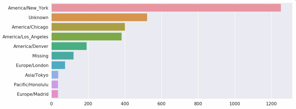
我們可以用matplotlib可視化這個數據。為此,我們先給記錄中未知或缺失的時區填上一個替代值。fillna函數可以替換缺失值(NA),而未知值(空字符串)則可以通過布爾型數組索引加以替換:
```python
In [31]: clean_tz = frame['tz'].fillna('Missing')
In [32]: clean_tz[clean_tz == ''] = 'Unknown'
In [33]: tz_counts = clean_tz.value_counts()
In [34]: tz_counts[:10]
Out[34]:
America/New_York 1251
Unknown 521
America/Chicago 400
America/Los_Angeles 382
America/Denver 191
Missing 120
Europe/London 74
Asia/Tokyo 37
Pacific/Honolulu 36
Europe/Madrid 35
Name: tz, dtype: int64
```
此時,我們可以用seaborn包創建水平柱狀圖(結果見圖14-1):
```python
In [36]: import seaborn as sns
In [37]: subset = tz_counts[:10]
In [38]: sns.barplot(y=subset.index, x=subset.values)
```
a字段含有執行URL短縮操作的瀏覽器、設備、應用程序的相關信息:
```python
In [39]: frame['a'][1]
Out[39]: 'GoogleMaps/RochesterNY'
In [40]: frame['a'][50]
Out[40]: 'Mozilla/5.0 (Windows NT 5.1; rv:10.0.2)
Gecko/20100101 Firefox/10.0.2'
In [41]: frame['a'][51][:50] # long line
Out[41]: 'Mozilla/5.0 (Linux; U; Android 2.2.2; en-us; LG-P9'
```
將這些"agent"字符串中的所有信息都解析出來是一件挺郁悶的工作。一種策略是將這種字符串的第一節(與瀏覽器大致對應)分離出來并得到另外一份用戶行為摘要:
```python
In [42]: results = pd.Series([x.split()[0] for x in frame.a.dropna()])
In [43]: results[:5]
Out[43]:
0 Mozilla/5.0
1 GoogleMaps/RochesterNY
2 Mozilla/4.0
3 Mozilla/5.0
4 Mozilla/5.0
dtype: object
In [44]: results.value_counts()[:8]
Out[44]:
Mozilla/5.0 2594
Mozilla/4.0 601
GoogleMaps/RochesterNY 121
Opera/9.80 34
TEST_INTERNET_AGENT 24
GoogleProducer 21
Mozilla/6.0 5
BlackBerry8520/5.0.0.681 4
dtype: int64
```
現在,假設你想按Windows和非Windows用戶對時區統計信息進行分解。為了簡單起見,我們假定只要agent字符串中含有"Windows"就認為該用戶為Windows用戶。由于有的agent缺失,所以首先將它們從數據中移除:
```python
In [45]: cframe = frame[frame.a.notnull()]
```
然后計算出各行是否含有Windows的值:
```python
In [47]: cframe['os'] = np.where(cframe['a'].str.contains('Windows'),
....: 'Windows', 'Not Windows')
In [48]: cframe['os'][:5]
Out[48]:
0 Windows
1 Not Windows
2 Windows
3 Not Windows
4 Windows
Name: os, dtype: object
```
接下來就可以根據時區和新得到的操作系統列表對數據進行分組了:
```python
In [49]: by_tz_os = cframe.groupby(['tz', 'os'])
```
分組計數,類似于value_counts函數,可以用size來計算。并利用unstack對計數結果進行重塑:
```python
In [50]: agg_counts = by_tz_os.size().unstack().fillna(0)
In [51]: agg_counts[:10]
Out[51]:
os Not Windows Windows
tz
245.0 276.0
Africa/Cairo 0.0 3.0
Africa/Casablanca 0.0 1.0
Africa/Ceuta 0.0 2.0
Africa/Johannesburg 0.0 1.0
Africa/Lusaka 0.0 1.0
America/Anchorage 4.0 1.0
America/Argentina/Buenos_Aires 1.0 0.0
America/Argentina/Cordoba 0.0 1.0
America/Argentina/Mendoza 0.0 1.0
```
最后,我們來選取最常出現的時區。為了達到這個目的,我根據agg_counts中的行數構造了一個間接索引數組:
```python
# Use to sort in ascending order
In [52]: indexer = agg_counts.sum(1).argsort()
In [53]: indexer[:10]
Out[53]:
tz
24
Africa/Cairo 20
Africa/Casablanca 21
Africa/Ceuta 92
Africa/Johannesburg 87
Africa/Lusaka 53
America/Anchorage 54
America/Argentina/Buenos_Aires 57
America/Argentina/Cordoba 26
America/Argentina/Mendoza 55
dtype: int64
```
然后我通過take按照這個順序截取了最后10行最大值:
```python
In [54]: count_subset = agg_counts.take(indexer[-10:])
In [55]: count_subset
Out[55]:
os Not Windows Windows
tz
America/Sao_Paulo 13.0 20.0
Europe/Madrid 16.0 19.0
Pacific/Honolulu 0.0 36.0
Asia/Tokyo 2.0 35.0
Europe/London 43.0 31.0
America/Denver 132.0 59.0
America/Los_Angeles 130.0 252.0
America/Chicago 115.0 285.0
245.0 276.0
America/New_York 339.0 912.0
```
pandas有一個簡便方法nlargest,可以做同樣的工作:
```python
In [56]: agg_counts.sum(1).nlargest(10)
Out[56]:
tz
America/New_York 1251.0
521.0
America/Chicago 400.0
America/Los_Angeles 382.0
America/Denver 191.0
Europe/London 74.0
Asia/Tokyo 37.0
Pacific/Honolulu 36.0
Europe/Madrid 35.0
America/Sao_Paulo 33.0
dtype: float64
```
然后,如這段代碼所示,可以用柱狀圖表示。我傳遞一個額外參數到seaborn的barpolt函數,來畫一個堆積條形圖(見圖14-2):
```python
# Rearrange the data for plotting
In [58]: count_subset = count_subset.stack()
In [59]: count_subset.name = 'total'
In [60]: count_subset = count_subset.reset_index()
In [61]: count_subset[:10]
Out[61]:
tz os total
0 America/Sao_Paulo Not Windows 13.0
1 America/Sao_Paulo Windows 20.0
2 Europe/Madrid Not Windows 16.0
3 Europe/Madrid Windows 19.0
4 Pacific/Honolulu Not Windows 0.0
5 Pacific/Honolulu Windows 36.0
6 Asia/Tokyo Not Windows 2.0
7 Asia/Tokyo Windows 35.0
8 Europe/London Not Windows 43.0
9 Europe/London Windows 31.0
In [62]: sns.barplot(x='total', y='tz', hue='os', data=count_subset)
```
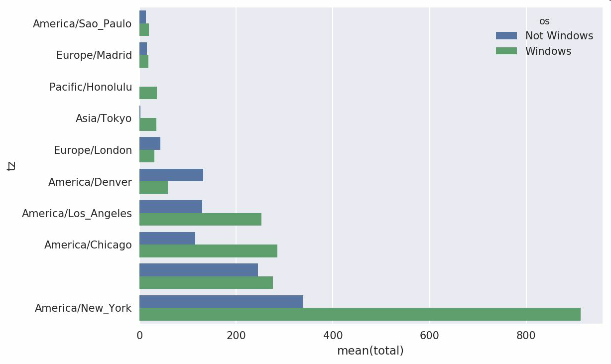
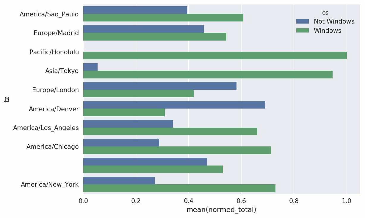
這張圖不容易看出Windows用戶在小分組中的相對比例,因此標準化分組百分比之和為1:
```python
def norm_total(group):
group['normed_total'] = group.total / group.total.sum()
return group
results = count_subset.groupby('tz').apply(norm_total)
```
再次畫圖,見圖14-3:
```python
In [65]: sns.barplot(x='normed_total', y='tz', hue='os', data=results)
```
我們還可以用groupby的transform方法,更高效的計算標準化的和:
```python
In [66]: g = count_subset.groupby('tz')
In [67]: results2 = count_subset.total / g.total.transform('sum')
```
# 14.2 MovieLens 1M數據集
GroupLens Research(http://www.grouplens.org/node/73)采集了一組從20世紀90年末到21世紀初由MovieLens用戶提供的電影評分數據。這些數據中包括電影評分、電影元數據(風格類型和年代)以及關于用戶的人口統計學數據(年齡、郵編、性別和職業等)。基于機器學習算法的推薦系統一般都會對此類數據感興趣。雖然我不會在本書中詳細介紹機器學習技術,但我會告訴你如何對這種數據進行切片切塊以滿足實際需求。
MovieLens 1M數據集含有來自6000名用戶對4000部電影的100萬條評分數據。它分為三個表:評分、用戶信息和電影信息。將該數據從zip文件中解壓出來之后,可以通過pandas.read_table將各個表分別讀到一個pandas DataFrame對象中:
```python
import pandas as pd
# Make display smaller
pd.options.display.max_rows = 10
unames = ['user_id', 'gender', 'age', 'occupation', 'zip']
users = pd.read_table('datasets/movielens/users.dat', sep='::',
header=None, names=unames)
rnames = ['user_id', 'movie_id', 'rating', 'timestamp']
ratings = pd.read_table('datasets/movielens/ratings.dat', sep='::',
header=None, names=rnames)
mnames = ['movie_id', 'title', 'genres']
movies = pd.read_table('datasets/movielens/movies.dat', sep='::',
header=None, names=mnames)
```
利用Python的切片語法,通過查看每個DataFrame的前幾行即可驗證數據加載工作是否一切順利:
```python
In [69]: users[:5]
Out[69]:
user_id gender age occupation zip
0 1 F 1 10 48067
1 2 M 56 16 70072
2 3 M 25 15 55117
3 4 M 45 7 02460
4 5 M 25 20 55455
In [70]: ratings[:5]
Out[70]:
user_id movie_id rating timestamp
0 1 1193 5 978300760
1 1 661 3 978302109
2 1 914 3 978301968
3 1 3408 4 978300275
4 1 2355 5 978824291
In [71]: movies[:5]
Out[71]:
movie_id title genres
0 1 Toy Story (1995) Animation|Children's|Comedy
1 2 Jumanji (1995) Adventure|Children's|Fantasy
2 3 Grumpier Old Men (1995) Comedy|Romance
3 4 Waiting to Exhale (1995) Comedy|Drama
4 5 Father of the Bride Part II (1995) Comedy
In [72]: ratings
Out[72]:
user_id movie_id rating timestamp
0 1 1193 5 978300760
1 1 661 3 978302109
2 1 914 3 978301968
3 1 3408 4 978300275
4 1 2355 5 978824291
... ... ... ... ...
1000204 6040 1091 1 956716541
1000205 6040 1094 5 956704887
1000206 6040 562 5 956704746
1000207 6040 1096 4 956715648
1000208 6040 1097 4 956715569
[1000209 rows x 4 columns]
```
注意,其中的年齡和職業是以編碼形式給出的,它們的具體含義請參考該數據集的README文件。分析散布在三個表中的數據可不是一件輕松的事情。假設我們想要根據性別和年齡計算某部電影的平均得分,如果將所有數據都合并到一個表中的話問題就簡單多了。我們先用pandas的merge函數將ratings跟users合并到一起,然后再將movies也合并進去。pandas會根據列名的重疊情況推斷出哪些列是合并(或連接)鍵:
```python
In [73]: data = pd.merge(pd.merge(ratings, users), movies)
In [74]: data
Out[74]:
user_id movie_id rating timestamp gender age occupation zip \
0 1 1193 5 978300760 F 1 10 48067
1 2 1193 5 978298413 M 56 16 70072
2 12 1193 4 978220179 M 25 12 32793
3 15 1193 4 978199279 M 25 7 22903
4 17 1193 5 978158471 M 50 1 95350
... ... ... ... ... ... ... ... ...
1000204 5949 2198 5 958846401 M 18 17 47901
1000205 5675 2703 3 976029116 M 35 14 30030
1000206 5780 2845 1 958153068 M 18 17 92886
1000207 5851 3607 5 957756608 F 18 20 55410
1000208 5938 2909 4 957273353 M 25 1 35401
title genres
0 One Flew Over the Cuckoo's Nest (1975) Drama
1 One Flew Over the Cuckoo's Nest (1975) Drama
2 One Flew Over the Cuckoo's Nest (1975) Drama
3 One Flew Over the Cuckoo's Nest (1975) Drama
4 One Flew Over the Cuckoo's Nest (1975) Drama
... ... ...
1000204 Modulations (1998) Documentary
1000205 Broken Vessels (1998) Drama
1000206 White Boys (1999) Drama
1000207 One Little Indian (1973) Comedy|Drama|Western
1000208 Five Wives, Three Secretaries and Me (1998) Documentary
[1000209 rows x 10 columns]
In [75]: data.iloc[0]
Out[75]:
user_id 1
movie_id 1193
rating 5
timestamp 978300760
gender F
age 1
occupation 10
zip 48067
title One Flew Over the Cuckoo's Nest (1975)
genres Drama
Name: 0, dtype: object
```
為了按性別計算每部電影的平均得分,我們可以使用pivot_table方法:
```python
In [76]: mean_ratings = data.pivot_table('rating', index='title',
....: columns='gender', aggfunc='mean')
In [77]: mean_ratings[:5]
Out[77]:
gender F M
title
$1,000,000 Duck (1971) 3.375000 2.761905
'Night Mother (1986) 3.388889 3.352941
'Til There Was You (1997) 2.675676 2.733333
'burbs, The (1989) 2.793478 2.962085
...And Justice for All (1979) 3.828571 3.689024
```
該操作產生了另一個DataFrame,其內容為電影平均得分,行標為電影名稱(索引),列標為性別。現在,我打算過濾掉評分數據不夠250條的電影(隨便選的一個數字)。為了達到這個目的,我先對title進行分組,然后利用size()得到一個含有各電影分組大小的Series對象:
```python
In [78]: ratings_by_title = data.groupby('title').size()
In [79]: ratings_by_title[:10]
Out[79]:
title
$1,000,000 Duck (1971) 37
'Night Mother (1986) 70
'Til There Was You (1997) 52
'burbs, The (1989) 303
...And Justice for All (1979) 199
1-900 (1994) 2
10 Things I Hate About You (1999) 700
101 Dalmatians (1961) 565
101 Dalmatians (1996) 364
12 Angry Men (1957) 616
dtype: int64
In [80]: active_titles = ratings_by_title.index[ratings_by_title >= 250]
In [81]: active_titles
Out[81]:
Index([''burbs, The (1989)', '10 Things I Hate About You (1999)',
'101 Dalmatians (1961)', '101 Dalmatians (1996)', '12 Angry Men (1957)',
'13th Warrior, The (1999)', '2 Days in the Valley (1996)',
'20,000 Leagues Under the Sea (1954)', '2001: A Space Odyssey (1968)',
'2010 (1984)',
...
'X-Men (2000)', 'Year of Living Dangerously (1982)',
'Yellow Submarine (1968)', 'You've Got Mail (1998)',
'Young Frankenstein (1974)', 'Young Guns (1988)',
'Young Guns II (1990)', 'Young Sherlock Holmes (1985)',
'Zero Effect (1998)', 'eXistenZ (1999)'],
dtype='object', name='title', length=1216)
```
標題索引中含有評分數據大于250條的電影名稱,然后我們就可以據此從前面的mean_ratings中選取所需的行了:
```python
# Select rows on the index
In [82]: mean_ratings = mean_ratings.loc[active_titles]
In [83]: mean_ratings
Out[83]:
gender F M
title
'burbs, The (1989) 2.793478 2.962085
10 Things I Hate About You (1999) 3.646552 3.311966
101 Dalmatians (1961) 3.791444 3.500000
101 Dalmatians (1996) 3.240000 2.911215
12 Angry Men (1957) 4.184397 4.328421
... ... ...
Young Guns (1988) 3.371795 3.425620
Young Guns II (1990) 2.934783 2.904025
Young Sherlock Holmes (1985) 3.514706 3.363344
Zero Effect (1998) 3.864407 3.723140
eXistenZ (1999) 3.098592 3.289086
[1216 rows x 2 columns]
```
為了了解女性觀眾最喜歡的電影,我們可以對F列降序排列:
```python
In [85]: top_female_ratings = mean_ratings.sort_values(by='F', ascending=False)
In [86]: top_female_ratings[:10]
Out[86]:
gender F M
title
Close Shave, A (1995) 4.644444 4.473795
Wrong Trousers, The (1993) 4.588235 4.478261
Sunset Blvd. (a.k.a. Sunset Boulevard) (1950) 4.572650 4.464589
Wallace & Gromit: The Best of Aardman Animation... 4.563107 4.385075
Schindler's List (1993) 4.562602 4.491415
Shawshank Redemption, The (1994) 4.539075 4.560625
Grand Day Out, A (1992) 4.537879 4.293255
To Kill a Mockingbird (1962) 4.536667 4.372611
Creature Comforts (1990) 4.513889 4.272277
Usual Suspects, The (1995) 4.513317 4.518248
```
## 計算評分分歧
假設我們想要找出男性和女性觀眾分歧最大的電影。一個辦法是給mean_ratings加上一個用于存放平均得分之差的列,并對其進行排序:
```python
In [87]: mean_ratings['diff'] = mean_ratings['M'] - mean_ratings['F']
```
按"diff"排序即可得到分歧最大且女性觀眾更喜歡的電影:
```python
In [88]: sorted_by_diff = mean_ratings.sort_values(by='diff')
In [89]: sorted_by_diff[:10]
Out[89]:
gender F M diff
title
Dirty Dancing (1987) 3.790378 2.959596 -0.830782
Jumpin' Jack Flash (1986) 3.254717 2.578358 -0.676359
Grease (1978) 3.975265 3.367041 -0.608224
Little Women (1994) 3.870588 3.321739 -0.548849
Steel Magnolias (1989) 3.901734 3.365957 -0.535777
Anastasia (1997) 3.800000 3.281609 -0.518391
Rocky Horror Picture Show, The (1975) 3.673016 3.160131 -0.512885
Color Purple, The (1985) 4.158192 3.659341 -0.498851
Age of Innocence, The (1993) 3.827068 3.339506 -0.487561
Free Willy (1993) 2.921348 2.438776 -0.482573
```
對排序結果反序并取出前10行,得到的則是男性觀眾更喜歡的電影:
```python
# Reverse order of rows, take first 10 rows
In [90]: sorted_by_diff[::-1][:10]
Out[90]:
gender F M diff
title
Good, The Bad and The Ugly, The (1966) 3.494949 4.221300 0.726351
Kentucky Fried Movie, The (1977) 2.878788 3.555147 0.676359
Dumb & Dumber (1994) 2.697987 3.336595 0.638608
Longest Day, The (1962) 3.411765 4.031447 0.619682
Cable Guy, The (1996) 2.250000 2.863787 0.613787
Evil Dead II (Dead By Dawn) (1987) 3.297297 3.909283 0.611985
Hidden, The (1987) 3.137931 3.745098 0.607167
Rocky III (1982) 2.361702 2.943503 0.581801
Caddyshack (1980) 3.396135 3.969737 0.573602
For a Few Dollars More (1965) 3.409091 3.953795 0.544704
```
如果只是想要找出分歧最大的電影(不考慮性別因素),則可以計算得分數據的方差或標準差:
```python
# Standard deviation of rating grouped by title
In [91]: rating_std_by_title = data.groupby('title')['rating'].std()
# Filter down to active_titles
In [92]: rating_std_by_title = rating_std_by_title.loc[active_titles]
# Order Series by value in descending order
In [93]: rating_std_by_title.sort_values(ascending=False)[:10]
Out[93]:
title
Dumb & Dumber (1994) 1.321333
Blair Witch Project, The (1999) 1.316368
Natural Born Killers (1994) 1.307198
Tank Girl (1995) 1.277695
Rocky Horror Picture Show, The (1975) 1.260177
Eyes Wide Shut (1999) 1.259624
Evita (1996) 1.253631
Billy Madison (1995) 1.249970
Fear and Loathing in Las Vegas (1998) 1.246408
Bicentennial Man (1999) 1.245533
Name: rating, dtype: float64
```
可能你已經注意到了,電影分類是以豎線(|)分隔的字符串形式給出的。如果想對電影分類進行分析的話,就需要先將其轉換成更有用的形式才行。
# 14.3 1880-2010年間全美嬰兒姓名
美國社會保障總署(SSA)提供了一份從1880年到現在的嬰兒名字頻率數據。Hadley Wickham(許多流行R包的作者)經常用這份數據來演示R的數據處理功能。
我們要做一些數據規整才能加載這個數據集,這么做就會產生一個如下的DataFrame:
```python
In [4]: names.head(10)
Out[4]:
name sex births year
0 Mary F 7065 1880
1 Anna F 2604 1880
2 Emma F 2003 1880
3 Elizabeth F 1939 1880
4 Minnie F 1746 1880
5 Margaret F 1578 1880
6 Ida F 1472 1880
7 Alice F 1414 1880
8 Bertha F 1320 1880
9 Sarah F 1288 1880
```
你可以用這個數據集做很多事,例如:
- 計算指定名字(可以是你自己的,也可以是別人的)的年度比例。
- 計算某個名字的相對排名。
- 計算各年度最流行的名字,以及增長或減少最快的名字。
- 分析名字趨勢:元音、輔音、長度、總體多樣性、拼寫變化、首尾字母等。
- 分析外源性趨勢:圣經中的名字、名人、人口結構變化等。
利用前面介紹過的那些工具,這些分析工作都能很輕松地完成,我會講解其中的一些。
到編寫本書時為止,美國社會保障總署將該數據庫按年度制成了多個數據文件,其中給出了每個性別/名字組合的出生總數。這些文件的原始檔案可以在這里獲取:[http://www.ssa.gov/oact/babynames/limits.html](http://www.ssa.gov/oact/babynames/limits.html)。
如果你在閱讀本書的時候這個頁面已經不見了,也可以用搜索引擎找找。
下載"National data"文件names.zip,解壓后的目錄中含有一組文件(如yob1880.txt)。我用UNIX的head命令查看了其中一個文件的前10行(在Windows上,你可以用more命令,或直接在文本編輯器中打開):
```
In [94]: !head -n 10 datasets/babynames/yob1880.txt
Mary,F,7065
Anna,F,2604
Emma,F,2003
Elizabeth,F,1939
Minnie,F,1746
Margaret,F,1578
Ida,F,1472
Alice,F,1414
Bertha,F,1320
Sarah,F,1288
```
由于這是一個非常標準的以逗號隔開的格式,所以可以用pandas.read_csv將其加載到DataFrame中:
```python
In [95]: import pandas as pd
In [96]: names1880 =
pd.read_csv('datasets/babynames/yob1880.txt',
....: names=['name', 'sex', 'births'])
In [97]: names1880
Out[97]:
name sex births
0 Mary F 7065
1 Anna F 2604
2 Emma F 2003
3 Elizabeth F 1939
4 Minnie F 1746
... ... .. ...
1995 Woodie M 5
1996 Worthy M 5
1997 Wright M 5
1998 York M 5
1999 Zachariah M 5
[2000 rows x 3 columns]
```
這些文件中僅含有當年出現超過5次的名字。為了簡單起見,我們可以用births列的sex分組小計表示該年度的births總計:
```python
In [98]: names1880.groupby('sex').births.sum()
Out[98]:
sex
F 90993
M 110493
Name: births, dtype: int64
```
由于該數據集按年度被分隔成了多個文件,所以第一件事情就是要將所有數據都組裝到一個DataFrame里面,并加上一個year字段。使用pandas.concat即可達到這個目的:
```python
years = range(1880, 2011)
pieces = []
columns = ['name', 'sex', 'births']
for year in years:
path = 'datasets/babynames/yob%d.txt' % year
frame = pd.read_csv(path, names=columns)
frame['year'] = year
pieces.append(frame)
# Concatenate everything into a single DataFrame
names = pd.concat(pieces, ignore_index=True)
```
這里需要注意幾件事情。第一,concat默認是按行將多個DataFrame組合到一起的;第二,必須指定ignore_index=True,因為我們不希望保留read_csv所返回的原始行號。現在我們得到了一個非常大的DataFrame,它含有全部的名字數據:
```python
In [100]: names
Out[100]:
name sex births year
0 Mary F 7065 1880
1 Anna F 2604 1880
2 Emma F 2003 1880
3 Elizabeth F 1939 1880
4 Minnie F 1746 1880
... ... .. ... ...
1690779 Zymaire M 5 2010
1690780 Zyonne M 5 2010
1690781 Zyquarius M 5 2010
1690782 Zyran M 5 2010
1690783 Zzyzx M 5 2010
[1690784 rows x 4 columns]
```
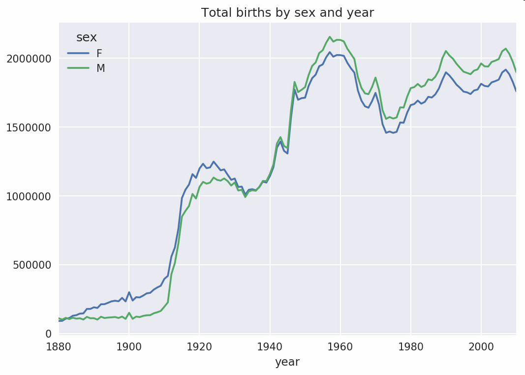
有了這些數據之后,我們就可以利用groupby或pivot_table在year和sex級別上對其進行聚合了,如圖14-4所示:
```python
In [101]: total_births = names.pivot_table('births', index='year',
.....: columns='sex', aggfunc=sum)
In [102]: total_births.tail()
Out[102]:
sex F M
year
2006 1896468 2050234
2007 1916888 2069242
2008 1883645 2032310
2009 1827643 1973359
2010 1759010 1898382
In [103]: total_births.plot(title='Total births by sex and year')
```
下面我們來插入一個prop列,用于存放指定名字的嬰兒數相對于總出生數的比例。prop值為0.02表示每100名嬰兒中有2名取了當前這個名字。因此,我們先按year和sex分組,然后再將新列加到各個分組上:
```python
def add_prop(group):
group['prop'] = group.births / group.births.sum()
return group
names = names.groupby(['year', 'sex']).apply(add_prop)
```
現在,完整的數據集就有了下面這些列:
```python
In [105]: names
Out[105]:
name sex births year prop
0 Mary F 7065 1880 0.077643
1 Anna F 2604 1880 0.028618
2 Emma F 2003 1880 0.022013
3 Elizabeth F 1939 1880 0.021309
4 Minnie F 1746 1880 0.019188
... ... .. ... ... ...
1690779 Zymaire M 5 2010 0.000003
1690780 Zyonne M 5 2010 0.000003
1690781 Zyquarius M 5 2010 0.000003
1690782 Zyran M 5 2010 0.000003
1690783 Zzyzx M 5 2010 0.000003
[1690784 rows x 5 columns]
```
在執行這樣的分組處理時,一般都應該做一些有效性檢查,比如驗證所有分組的prop的總和是否為1:
```python
In [106]: names.groupby(['year', 'sex']).prop.sum()
Out[106]:
year sex
1880 F 1.0
M 1.0
1881 F 1.0
M 1.0
1882 F 1.0
...
2008 M 1.0
2009 F 1.0
M 1.0
2010 F 1.0
M 1.0
Name: prop, Length: 262, dtype: float64
```
工作完成。為了便于實現更進一步的分析,我需要取出該數據的一個子集:每對sex/year組合的前1000個名字。這又是一個分組操作:
```python
def get_top1000(group):
return group.sort_values(by='births', ascending=False)[:1000]
grouped = names.groupby(['year', 'sex'])
top1000 = grouped.apply(get_top1000)
# Drop the group index, not needed
top1000.reset_index(inplace=True, drop=True)
```
如果你喜歡DIY的話,也可以這樣:
```python
pieces = []
for year, group in names.groupby(['year', 'sex']):
pieces.append(group.sort_values(by='births', ascending=False)[:1000])
top1000 = pd.concat(pieces, ignore_index=True)
```
現在的結果數據集就小多了:
```python
In [108]: top1000
Out[108]:
name sex births year prop
0 Mary F 7065 1880 0.077643
1 Anna F 2604 1880 0.028618
2 Emma F 2003 1880 0.022013
3 Elizabeth F 1939 1880 0.021309
4 Minnie F 1746 1880 0.019188
... ... .. ... ... ...
261872 Camilo M 194 2010 0.000102
261873 Destin M 194 2010 0.000102
261874 Jaquan M 194 2010 0.000102
261875 Jaydan M 194 2010 0.000102
261876 Maxton M 193 2010 0.000102
[261877 rows x 5 columns]
```
接下來的數據分析工作就針對這個top1000數據集了。
## 分析命名趨勢
有了完整的數據集和剛才生成的top1000數據集,我們就可以開始分析各種命名趨勢了。首先將前1000個名字分為男女兩個部分:
```python
In [109]: boys = top1000[top1000.sex == 'M']
In [110]: girls = top1000[top1000.sex == 'F']
```
這是兩個簡單的時間序列,只需稍作整理即可繪制出相應的圖表(比如每年叫做John和Mary的嬰兒數)。我們先生成一張按year和name統計的總出生數透視表:
```python
In [111]: total_births = top1000.pivot_table('births', index='year',
.....: columns='name',
.....: aggfunc=sum)
```
現在,我們用DataFrame的plot方法繪制幾個名字的曲線圖(見圖14-5):
```python
In [112]: total_births.info()
<class 'pandas.core.frame.DataFrame'>
Int64Index: 131 entries, 1880 to 2010
Columns: 6868 entries, Aaden to Zuri
dtypes: float64(6868)
memory usage: 6.9 MB
In [113]: subset = total_births[['John', 'Harry', 'Mary', 'Marilyn']]
In [114]: subset.plot(subplots=True, figsize=(12, 10), grid=False,
.....: title="Number of births per year")
```
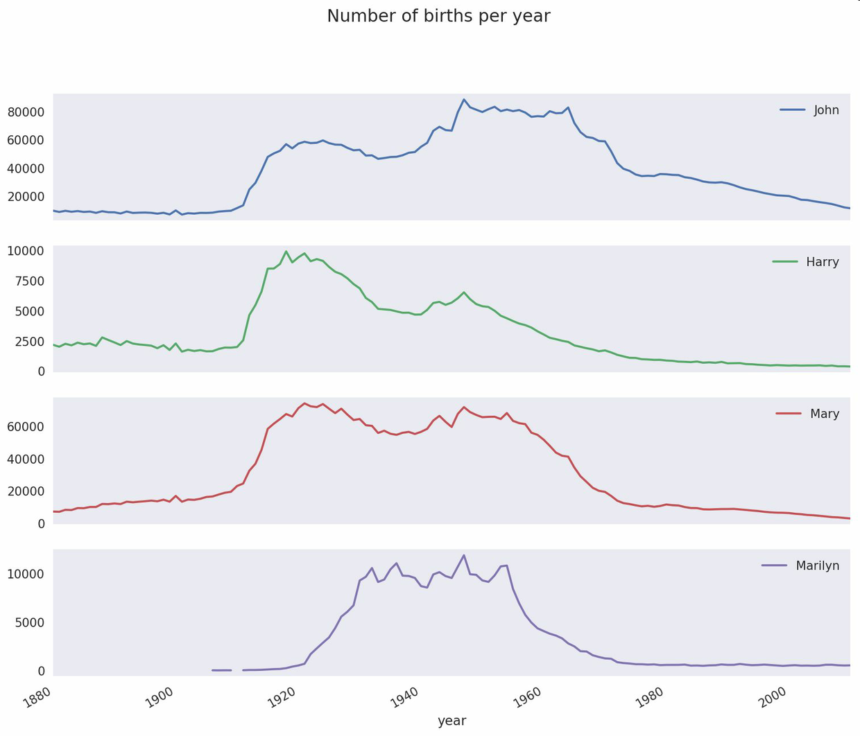
從圖中可以看出,這幾個名字在美國人民的心目中已經風光不再了。但事實并非如此簡單,我們在下一節中就能知道是怎么一回事了。
## 評估命名多樣性的增長
一種解釋是父母愿意給小孩起常見的名字越來越少。這個假設可以從數據中得到驗證。一個辦法是計算最流行的1000個名字所占的比例,我按year和sex進行聚合并繪圖(見圖14-6):
```python
In [116]: table = top1000.pivot_table('prop', index='year',
.....: columns='sex', aggfunc=sum)
In [117]: table.plot(title='Sum of table1000.prop by year and sex',
.....: yticks=np.linspace(0, 1.2, 13), xticks=range(1880, 2020, 10)
)
```
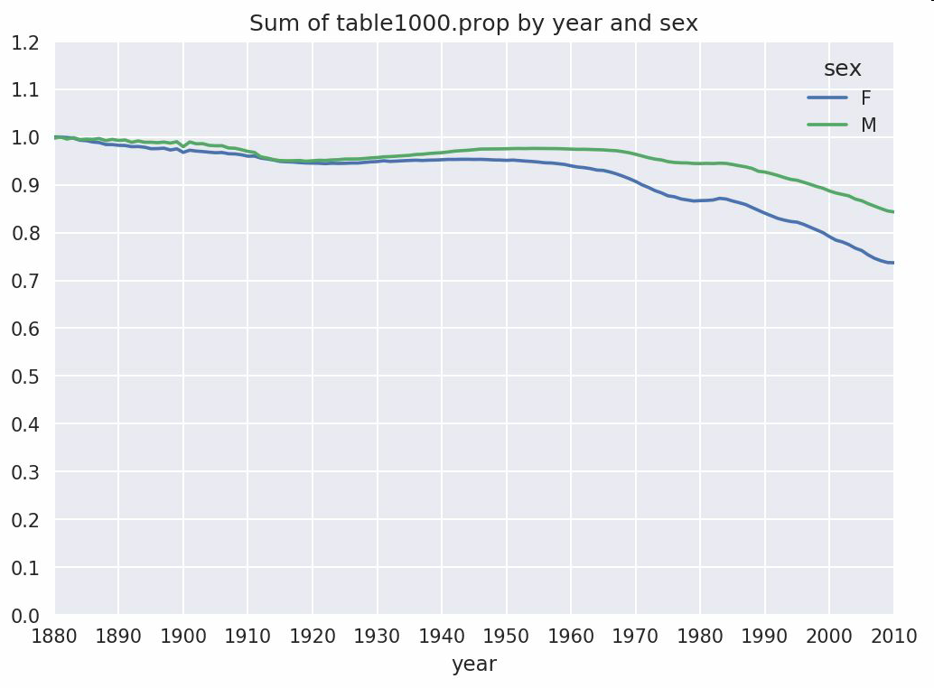
從圖中可以看出,名字的多樣性確實出現了增長(前1000項的比例降低)。另一個辦法是計算占總出生人數前50%的不同名字的數量,這個數字不太好計算。我們只考慮2010年男孩的名字:
```python
In [118]: df = boys[boys.year == 2010]
In [119]: df
Out[119]:
name sex births year prop
260877 Jacob M 21875 2010 0.011523
260878 Ethan M 17866 2010 0.009411
260879 Michael M 17133 2010 0.009025
260880 Jayden M 17030 2010 0.008971
260881 William M 16870 2010 0.008887
... ... .. ... ... ...
261872 Camilo M 194 2010 0.000102
261873 Destin M 194 2010 0.000102
261874 Jaquan M 194 2010 0.000102
261875 Jaydan M 194 2010 0.000102
261876 Maxton M 193 2010 0.000102
[1000 rows x 5 columns]
```
在對prop降序排列之后,我們想知道前面多少個名字的人數加起來才夠50%。雖然編寫一個for循環確實也能達到目的,但NumPy有一種更聰明的矢量方式。先計算prop的累計和cumsum,然后再通過searchsorted方法找出0.5應該被插入在哪個位置才能保證不破壞順序:
```python
In [120]: prop_cumsum = df.sort_values(by='prop', ascending=False).prop.cumsum()
In [121]: prop_cumsum[:10]
Out[121]:
260877 0.011523
260878 0.020934
260879 0.029959
260880 0.038930
260881 0.047817
260882 0.056579
260883 0.065155
260884 0.073414
260885 0.081528
260886 0.089621
Name: prop, dtype: float64
In [122]: prop_cumsum.values.searchsorted(0.5)
Out[122]: 116
```
由于數組索引是從0開始的,因此我們要給這個結果加1,即最終結果為117。拿1900年的數據來做個比較,這個數字要小得多:
```python
In [123]: df = boys[boys.year == 1900]
In [124]: in1900 = df.sort_values(by='prop', ascending=False).prop.cumsum()
In [125]: in1900.values.searchsorted(0.5) + 1
Out[125]: 25
```
現在就可以對所有year/sex組合執行這個計算了。按這兩個字段進行groupby處理,然后用一個函數計算各分組的這個值:
```python
def get_quantile_count(group, q=0.5):
group = group.sort_values(by='prop', ascending=False)
return group.prop.cumsum().values.searchsorted(q) + 1
diversity = top1000.groupby(['year', 'sex']).apply(get_quantile_count)
diversity = diversity.unstack('sex')
```
現在,diversity這個DataFrame擁有兩個時間序列(每個性別各一個,按年度索引)。通過IPython,你可以查看其內容,還可以像之前那樣繪制圖表(如圖14-7所示):
```python
In [128]: diversity.head()
Out[128]:
sex F M
year
1880 38 14
1881 38 14
1882 38 15
1883 39 15
1884 39 16
In [129]: diversity.plot(title="Number of popular names in top 50%")
```
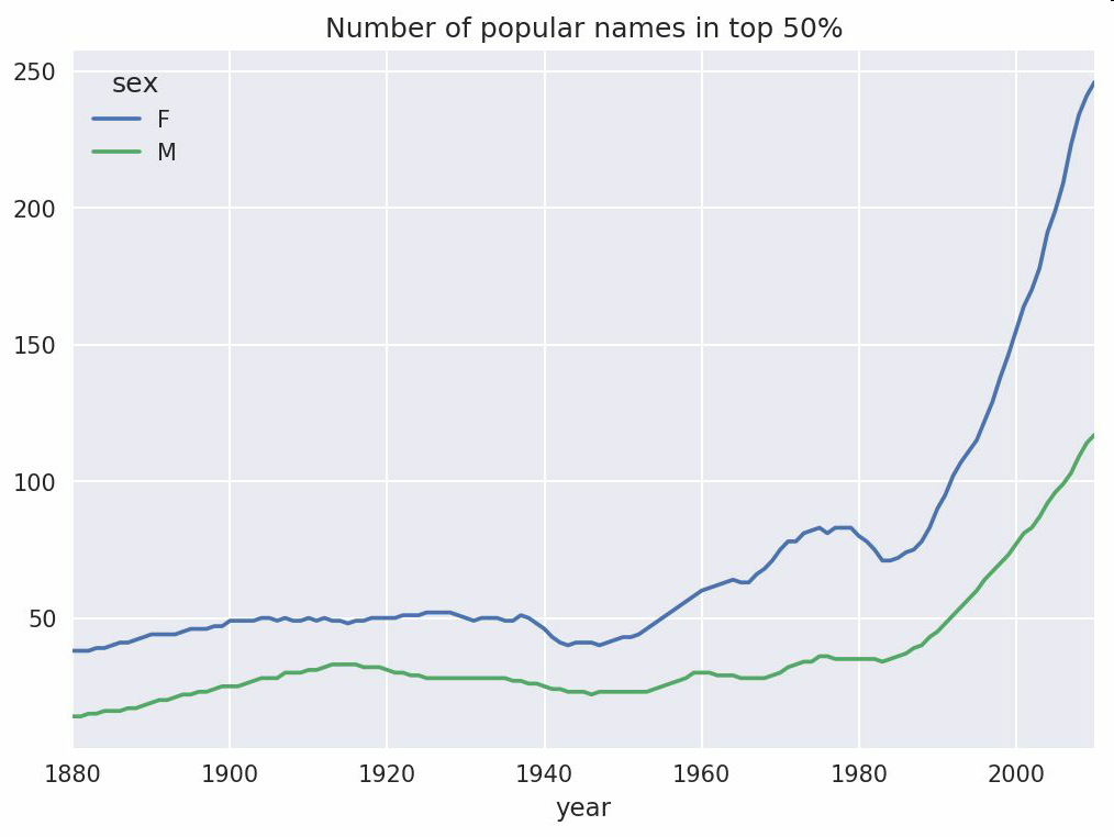
從圖中可以看出,女孩名字的多樣性總是比男孩的高,而且還在變得越來越高。讀者們可以自己分析一下具體是什么在驅動這個多樣性(比如拼寫形式的變化)。
## “最后一個字母”的變革
2007年,一名嬰兒姓名研究人員Laura Wattenberg在她自己的網站上指出(http://www.babynamewizard.com):近百年來,男孩名字在最后一個字母上的分布發生了顯著的變化。為了了解具體的情況,我首先將全部出生數據在年度、性別以及末字母上進行了聚合:
```python
# extract last letter from name column
get_last_letter = lambda x: x[-1]
last_letters = names.name.map(get_last_letter)
last_letters.name = 'last_letter'
table = names.pivot_table('births', index=last_letters,
columns=['sex', 'year'], aggfunc=sum)
```
然后,我選出具有一定代表性的三年,并輸出前面幾行:
```python
In [131]: subtable = table.reindex(columns=[1910, 1960, 2010], level='year')
In [132]: subtable.head()
Out[132]:
sex F M
year 1910 1960 2010 1910 1960 2010
last_letter
a 108376.0 691247.0 670605.0 977.0 5204.0 28438.0
b NaN 694.0 450.0 411.0 3912.0 38859.0
c 5.0 49.0 946.0 482.0 15476.0 23125.0
d 6750.0 3729.0 2607.0 22111.0 262112.0 44398.0
e 133569.0 435013.0 313833.0 28655.0 178823.0 129012.0
```
接下來我們需要按總出生數對該表進行規范化處理,以便計算出各性別各末字母占總出生人數的比例:
```python
In [133]: subtable.sum()
Out[133]:
sex year
F 1910 396416.0
1960 2022062.0
2010 1759010.0
M 1910 194198.0
1960 2132588.0
2010 1898382.0
dtype: float64
In [134]: letter_prop = subtable / subtable.sum()
In [135]: letter_prop
Out[135]:
sex F M
year 1910 1960 2010 1910 1960 2010
last_letter
a 0.273390 0.341853 0.381240 0.005031 0.002440 0.014980
b NaN 0.000343 0.000256 0.002116 0.001834 0.020470
c 0.000013 0.000024 0.000538 0.002482 0.007257 0.012181
d 0.017028 0.001844 0.001482 0.113858 0.122908 0.023387
e 0.336941 0.215133 0.178415 0.147556 0.083853 0.067959
... ... ... ... ... ... ...
v NaN 0.000060 0.000117 0.000113
0.000037 0.001434
w 0.000020 0.000031 0.001182 0.006329 0.007711 0.016148
x 0.000015 0.000037 0.000727 0.003965 0.001851 0.008614
y 0.110972 0.152569 0.116828 0.077349 0.160987 0.058168
z 0.002439 0.000659 0.000704 0.000170 0.000184 0.001831
[26 rows x 6 columns]
```
有了這個字母比例數據之后,就可以生成一張各年度各性別的條形圖了,如圖14-8所示:
```python
import matplotlib.pyplot as plt
fig, axes = plt.subplots(2, 1, figsize=(10, 8))
letter_prop['M'].plot(kind='bar', rot=0, ax=axes[0], title='Male')
letter_prop['F'].plot(kind='bar', rot=0, ax=axes[1], title='Female',
legend=False)
```
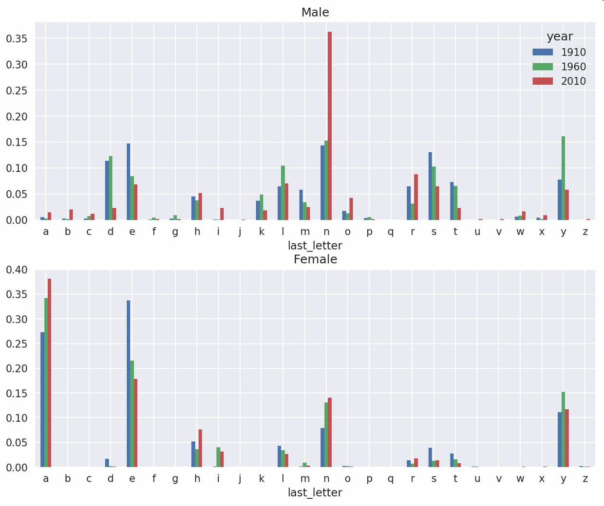
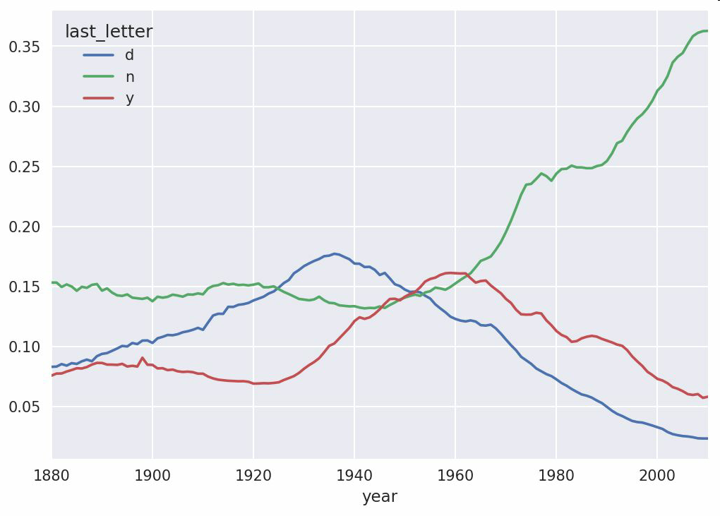
可以看出,從20世紀60年代開始,以字母"n"結尾的男孩名字出現了顯著的增長。回到之前創建的那個完整表,按年度和性別對其進行規范化處理,并在男孩名字中選取幾個字母,最后進行轉置以便將各個列做成一個時間序列:
```python
In [138]: letter_prop = table / table.sum()
In [139]: dny_ts = letter_prop.loc[['d', 'n', 'y'], 'M'].T
In [140]: dny_ts.head()
Out[140]:
last_letter d n y
year
1880 0.083055 0.153213 0.075760
1881 0.083247 0.153214 0.077451
1882 0.085340 0.149560 0.077537
1883 0.084066 0.151646 0.079144
1884 0.086120 0.149915 0.080405
```
有了這個時間序列的DataFrame之后,就可以通過其plot方法繪制出一張趨勢圖了(如圖14-9所示):
```python
In [143]: dny_ts.plot()
```
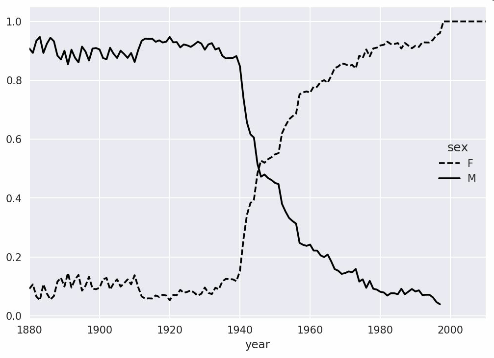
## 變成女孩名字的男孩名字(以及相反的情況)
另一個有趣的趨勢是,早年流行于男孩的名字近年來“變性了”,例如Lesley或Leslie。回到top1000數據集,找出其中以"lesl"開頭的一組名字:
```python
In [144]: all_names = pd.Series(top1000.name.unique())
In [145]: lesley_like = all_names[all_names.str.lower().str.contains('lesl')]
In [146]: lesley_like
Out[146]:
632 Leslie
2294 Lesley
4262 Leslee
4728 Lesli
6103 Lesly
dtype: object
```
然后利用這個結果過濾其他的名字,并按名字分組計算出生數以查看相對頻率:
```python
In [147]: filtered = top1000[top1000.name.isin(lesley_like)]
In [148]: filtered.groupby('name').births.sum()
Out[148]:
name
Leslee 1082
Lesley 35022
Lesli 929
Leslie 370429
Lesly 10067
Name: births, dtype: int64
```
接下來,我們按性別和年度進行聚合,并按年度進行規范化處理:
```python
In [149]: table = filtered.pivot_table('births', index='year',
.....: columns='sex', aggfunc='sum')
In [150]: table = table.div(table.sum(1), axis=0)
In [151]: table.tail()
Out[151]:
sex F M
year
2006 1.0 NaN
2007 1.0 NaN
2008 1.0 NaN
2009 1.0 NaN
2010 1.0 NaN
```
最后,就可以輕松繪制一張分性別的年度曲線圖了(如圖2-10所示):
```python
In [153]: table.plot(style={'M': 'k-', 'F': 'k--'})
```
# 14.4 USDA食品數據庫
美國農業部(USDA)制作了一份有關食物營養信息的數據庫。Ashley Williams制作了該數據的JSON版(http://ashleyw.co.uk/project/food-nutrient-database)。其中的記錄如下所示:
```python
{
"id": 21441,
"description": "KENTUCKY FRIED CHICKEN, Fried Chicken, EXTRA CRISPY,
Wing, meat and skin with breading",
"tags": ["KFC"],
"manufacturer": "Kentucky Fried Chicken",
"group": "Fast Foods",
"portions": [
{
"amount": 1,
"unit": "wing, with skin",
"grams": 68.0
},
...
],
"nutrients": [
{
"value": 20.8,
"units": "g",
"description": "Protein",
"group": "Composition"
},
...
]
}
```
每種食物都帶有若干標識性屬性以及兩個有關營養成分和分量的列表。這種形式的數據不是很適合分析工作,因此我們需要做一些規整化以使其具有更好用的形式。
從上面列舉的那個網址下載并解壓數據之后,你可以用任何喜歡的JSON庫將其加載到Python中。我用的是Python內置的json模塊:
```python
In [154]: import json
In [155]: db = json.load(open('datasets/usda_food/database.json'))
In [156]: len(db)
Out[156]: 6636
```
db中的每個條目都是一個含有某種食物全部數據的字典。nutrients字段是一個字典列表,其中的每個字典對應一種營養成分:
```python
In [157]: db[0].keys()
Out[157]: dict_keys(['id', 'description', 'tags', 'manufacturer', 'group', 'porti
ons', 'nutrients'])
In [158]: db[0]['nutrients'][0]
Out[158]:
{'description': 'Protein',
'group': 'Composition',
'units': 'g',
'value': 25.18}
In [159]: nutrients = pd.DataFrame(db[0]['nutrients'])
In [160]: nutrients[:7]
Out[160]:
description group units value
0 Protein Composition g 25.18
1 Total lipid (fat) Composition g 29.20
2 Carbohydrate, by difference Composition g 3.06
3 Ash Other g 3.28
4 Energy Energy kcal 376.00
5 Water Composition g 39.28
6 Energy Energy kJ 1573.00
```
在將字典列表轉換為DataFrame時,可以只抽取其中的一部分字段。這里,我們將取出食物的名稱、分類、編號以及制造商等信息:
```python
In [161]: info_keys = ['description', 'group', 'id', 'manufacturer']
In [162]: info = pd.DataFrame(db, columns=info_keys)
In [163]: info[:5]
Out[163]:
description group id \
0 Cheese, caraway Dairy and Egg Products 1008
1 Cheese, cheddar Dairy and Egg Products 1009
2 Cheese, edam Dairy and Egg Products 1018
3 Cheese, feta Dairy and Egg Products 1019
4 Cheese, mozzarella, part skim milk Dairy and Egg Products 1028
manufacturer
0
1
2
3
4
In [164]: info.info()
<class 'pandas.core.frame.DataFrame'>
RangeIndex: 6636 entries, 0 to 6635
Data columns (total 4 columns):
description 6636 non-null object
group 6636 non-null object
id 6636 non-null int64
manufacturer 5195 non-null object
dtypes: int64(1), object(3)
memory usage: 207.5+ KB
```
通過value_counts,你可以查看食物類別的分布情況:
```python
In [165]: pd.value_counts(info.group)[:10]
Out[165]:
Vegetables and Vegetable Products 812
Beef Products 618
Baked Products 496
Breakfast Cereals 403
Fast Foods 365
Legumes and Legume Products 365
Lamb, Veal, and Game Products 345
Sweets 341
Pork Products 328
Fruits and Fruit Juices 328
Name: group, dtype: int64
```
現在,為了對全部營養數據做一些分析,最簡單的辦法是將所有食物的營養成分整合到一個大表中。我們分幾個步驟來實現該目的。首先,將各食物的營養成分列表轉換為一個DataFrame,并添加一個表示編號的列,然后將該DataFrame添加到一個列表中。最后通過concat將這些東西連接起來就可以了:
順利的話,nutrients的結果是:
```python
In [167]: nutrients
Out[167]:
description group units value id
0 Protein Composition g 25.180 1008
1 Total lipid (fat) Composition g 29.200 1008
2 Carbohydrate, by difference Composition g 3.060 1008
3 Ash Other g 3.280 1008
4 Energy Energy kcal 376.000 1008
... ... ...
... ... ...
389350 Vitamin B-12, added Vitamins mcg 0.000 43546
389351 Cholesterol Other mg 0.000 43546
389352 Fatty acids, total saturated Other g 0.072 43546
389353 Fatty acids, total monounsaturated Other g 0.028 43546
389354 Fatty acids, total polyunsaturated Other g 0.041 43546
[389355 rows x 5 columns]
```
我發現這個DataFrame中無論如何都會有一些重復項,所以直接丟棄就可以了:
```python
In [168]: nutrients.duplicated().sum() # number of duplicates
Out[168]: 14179
In [169]: nutrients = nutrients.drop_duplicates()
```
由于兩個DataFrame對象中都有"group"和"description",所以為了明確到底誰是誰,我們需要對它們進行重命名:
```python
In [170]: col_mapping = {'description' : 'food',
.....: 'group' : 'fgroup'}
In [171]: info = info.rename(columns=col_mapping, copy=False)
In [172]: info.info()
<class 'pandas.core.frame.DataFrame'>
RangeIndex: 6636 entries, 0 to 6635
Data columns (total 4 columns):
food 6636 non-null object
fgroup 6636 non-null object
id 6636 non-null int64
manufacturer 5195 non-null object
dtypes: int64(1), object(3)
memory usage: 207.5+ KB
In [173]: col_mapping = {'description' : 'nutrient',
.....: 'group' : 'nutgroup'}
In [174]: nutrients = nutrients.rename(columns=col_mapping, copy=False)
In [175]: nutrients
Out[175]:
nutrient nutgroup units value id
0 Protein Composition g 25.180 1008
1 Total lipid (fat) Composition g 29.200 1008
2 Carbohydrate, by difference Composition g 3.060 1008
3 Ash Other g 3.280 1008
4 Energy Energy kcal 376.000 1008
... ... ... ... ... ...
389350 Vitamin B-12, added Vitamins mcg 0.000 43546
389351 Cholesterol Other mg 0.000 43546
389352 Fatty acids, total saturated Other g 0.072 43546
389353 Fatty acids, total monounsaturated Other g 0.028 43546
389354 Fatty acids, total polyunsaturated Other g 0.041 43546
[375176 rows x 5 columns]
```
做完這些,就可以將info跟nutrients合并起來:
```python
In [176]: ndata = pd.merge(nutrients, info, on='id', how='outer')
In [177]: ndata.info()
<class 'pandas.core.frame.DataFrame'>
Int64Index: 375176 entries, 0 to 375175
Data columns (total 8 columns):
nutrient 375176 non-null object
nutgroup 375176 non-null object
units 375176 non-null object
value 375176 non-null float64
id 375176 non-null int64
food 375176 non-null object
fgroup 375176 non-null object
manufacturer 293054 non-null object
dtypes: float64(1), int64(1), object(6)
memory usage: 25.8+ MB
In [178]: ndata.iloc[30000]
Out[178]:
nutrient Glycine
nutgroup Amino Acids
units g
value 0.04
id 6158
food Soup, tomato bisque, canned, condensed
fgroup Soups, Sauces, and Gravies
manufacturer
Name: 30000, dtype: object
```
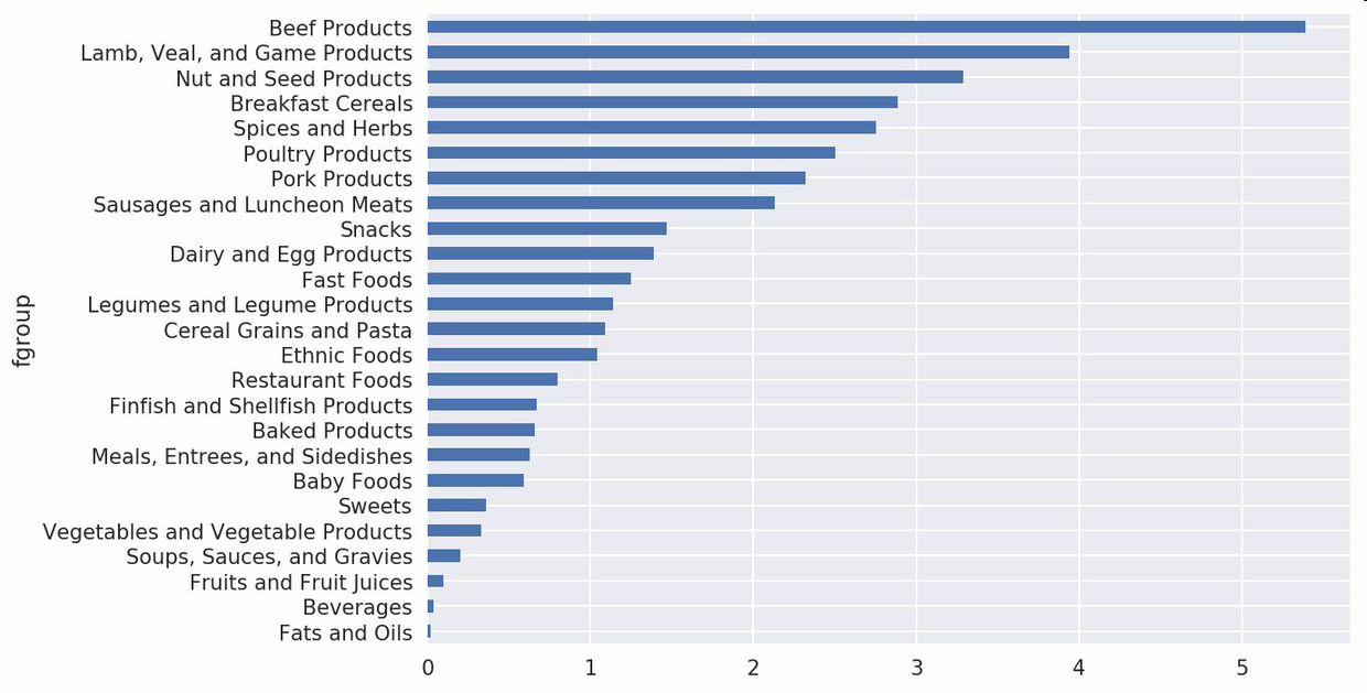
我們現在可以根據食物分類和營養類型畫出一張中位值圖(如圖14-11所示):
```python
In [180]: result = ndata.groupby(['nutrient', 'fgroup'])['value'].quantile(0.5)
In [181]: result['Zinc, Zn'].sort_values().plot(kind='barh')
```
只要稍微動一動腦子,就可以發現各營養成分最為豐富的食物是什么了:
```python
by_nutrient = ndata.groupby(['nutgroup', 'nutrient'])
get_maximum = lambda x: x.loc[x.value.idxmax()]
get_minimum = lambda x: x.loc[x.value.idxmin()]
max_foods = by_nutrient.apply(get_maximum)[['value', 'food']]
# make the food a little smaller
max_foods.food = max_foods.food.str[:50]
```
由于得到的DataFrame很大,所以不方便在書里面全部打印出來。這里只給出"Amino Acids"營養分組:
```python
In [183]: max_foods.loc['Amino Acids']['food']
Out[183]:
nutrient
Alanine Gelatins, dry powder, unsweetened
Arginine Seeds, sesame flour, low-fat
Aspartic acid Soy protein isolate
Cystine Seeds, cottonseed flour, low fat (glandless)
Glutamic acid Soy protein isolate
...
Serine Soy protein isolate, PROTEIN TECHNOLOGIES INTE...
Threonine Soy protein isolate, PROTEIN TECHNOLOGIES INTE...
Tryptophan Sea lion, Steller, meat with fat (Alaska Native)
Tyrosine Soy protein isolate, PROTEIN TECHNOLOGIES INTE...
Valine Soy protein isolate, PROTEIN TECHNOLOGIES INTE...
Name: food, Length: 19, dtype: object
```
# 14.5 2012聯邦選舉委員會數據庫
美國聯邦選舉委員會發布了有關政治競選贊助方面的數據。其中包括贊助者的姓名、職業、雇主、地址以及出資額等信息。我們對2012年美國總統大選的數據集比較感興趣(http://www.fec.gov/disclosurep/PDownload.do)。我在2012年6月下載的數據集是一個150MB的CSV文件(P00000001-ALL.csv),我們先用pandas.read_csv將其加載進來:
```python
In [184]: fec = pd.read_csv('datasets/fec/P00000001-ALL.csv')
In [185]: fec.info()
<class 'pandas.core.frame.DataFrame'>
RangeIndex: 1001731 entries, 0 to 1001730
Data columns (total 16 columns):
cmte_id 1001731 non-null object
cand_id 1001731 non-null object
cand_nm 1001731 non-null object
contbr_nm 1001731 non-null object
contbr_city 1001712 non-null object
contbr_st 1001727 non-null object
contbr_zip 1001620 non-null object
contbr_employer 988002 non-null object
contbr_occupation 993301 non-null object
contb_receipt_amt 1001731 non-null float64
contb_receipt_dt 1001731 non-null object
receipt_desc 14166 non-null object
memo_cd 92482 non-null object
memo_text 97770 non-null object
form_tp 1001731 non-null object
file_num 1001731 non-null int64
dtypes: float64(1), int64(1), object(14)
memory usage: 122.3+ MB
```
該DataFrame中的記錄如下所示:
```python
In [186]: fec.iloc[123456]
Out[186]:
cmte_id C00431445
cand_id P80003338
cand_nm Obama, Barack
contbr_nm ELLMAN, IRA
contbr_city TEMPE
...
receipt_desc NaN
memo_cd NaN
memo_text NaN
form_tp SA17A
file_num 772372
Name: 123456, Length: 16, dtype: object
```
你可能已經想出了許多辦法從這些競選贊助數據中抽取有關贊助人和贊助模式的統計信息。我將在接下來的內容中介紹幾種不同的分析工作(運用到目前為止已經學到的方法)。
不難看出,該數據中沒有黨派信息,因此最好把它加進去。通過unique,你可以獲取全部的候選人名單:
```python
In [187]: unique_cands = fec.cand_nm.unique()
In [188]: unique_cands
Out[188]:
array(['Bachmann, Michelle', 'Romney, Mitt', 'Obama, Barack',
"Roemer, Charles E. 'Buddy' III", 'Pawlenty, Timothy',
'Johnson, Gary Earl', 'Paul, Ron', 'Santorum, Rick', 'Cain, Herman',
'Gingrich, Newt', 'McCotter, Thaddeus G', 'Huntsman, Jon',
'Perry, Rick'], dtype=object)
In [189]: unique_cands[2]
Out[189]: 'Obama, Barack'
```
指明黨派信息的方法之一是使用字典:
```python
parties = {'Bachmann, Michelle': 'Republican',
'Cain, Herman': 'Republican',
'Gingrich, Newt': 'Republican',
'Huntsman, Jon': 'Republican',
'Johnson, Gary Earl': 'Republican',
'McCotter, Thaddeus G': 'Republican',
'Obama, Barack': 'Democrat',
'Paul, Ron': 'Republican',
'Pawlenty, Timothy': 'Republican',
'Perry, Rick': 'Republican',
"Roemer, Charles E. 'Buddy' III": 'Republican',
'Romney, Mitt': 'Republican',
'Santorum, Rick': 'Republican'}
```
現在,通過這個映射以及Series對象的map方法,你可以根據候選人姓名得到一組黨派信息:
```python
In [191]: fec.cand_nm[123456:123461]
Out[191]:
123456 Obama, Barack
123457 Obama, Barack
123458 Obama, Barack
123459 Obama, Barack
123460 Obama, Barack
Name: cand_nm, dtype: object
In [192]: fec.cand_nm[123456:123461].map(parties)
Out[192]:
123456 Democrat
123457 Democrat
123458 Democrat
123459 Democrat
123460 Democrat
Name: cand_nm, dtype: object
# Add it as a column
In [193]: fec['party'] = fec.cand_nm.map(parties)
In [194]: fec['party'].value_counts()
Out[194]:
Democrat 593746
Republican 407985
Name: party, dtype: int64
```
這里有兩個需要注意的地方。第一,該數據既包括贊助也包括退款(負的出資額):
```python
In [195]: (fec.contb_receipt_amt > 0).value_counts()
Out[195]:
True 991475
False 10256
Name: contb_receipt_amt, dtype: int64
```
為了簡化分析過程,我限定該數據集只能有正的出資額:
```python
In [196]: fec = fec[fec.contb_receipt_amt > 0]
```
由于Barack Obama和Mitt Romney是最主要的兩名候選人,所以我還專門準備了一個子集,只包含針對他們兩人的競選活動的贊助信息:
```python
In [197]: fec_mrbo = fec[fec.cand_nm.isin(['Obama, Barack','Romney, Mitt'])]
```
## 根據職業和雇主統計贊助信息
基于職業的贊助信息統計是另一種經常被研究的統計任務。例如,律師們更傾向于資助民主黨,而企業主則更傾向于資助共和黨。你可以不相信我,自己看那些數據就知道了。首先,根據職業計算出資總額,這很簡單:
```python
In [198]: fec.contbr_occupation.value_counts()[:10]
Out[198]:
RETIRED 233990
INFORMATION REQUESTED 35107
ATTORNEY 34286
HOMEMAKER 29931
PHYSICIAN 23432
INFORMATION REQUESTED PER BEST EFFORTS 21138
ENGINEER 14334
TEACHER 13990
CONSULTANT 13273
PROFESSOR 12555
Name: contbr_occupation, dtype: int64
```
不難看出,許多職業都涉及相同的基本工作類型,或者同一樣東西有多種變體。下面的代碼片段可以清理一些這樣的數據(將一個職業信息映射到另一個)。注意,這里巧妙地利用了dict.get,它允許沒有映射關系的職業也能“通過”:
```python
occ_mapping = {
'INFORMATION REQUESTED PER BEST EFFORTS' : 'NOT PROVIDED',
'INFORMATION REQUESTED' : 'NOT PROVIDED',
'INFORMATION REQUESTED (BEST EFFORTS)' : 'NOT PROVIDED',
'C.E.O.': 'CEO'
}
# If no mapping provided, return x
f = lambda x: occ_mapping.get(x, x)
fec.contbr_occupation = fec.contbr_occupation.map(f)
```
我對雇主信息也進行了同樣的處理:
```python
emp_mapping = {
'INFORMATION REQUESTED PER BEST EFFORTS' : 'NOT PROVIDED',
'INFORMATION REQUESTED' : 'NOT PROVIDED',
'SELF' : 'SELF-EMPLOYED',
'SELF EMPLOYED' : 'SELF-EMPLOYED',
}
# If no mapping provided, return x
f = lambda x: emp_mapping.get(x, x)
fec.contbr_employer = fec.contbr_employer.map(f)
```
現在,你可以通過pivot_table根據黨派和職業對數據進行聚合,然后過濾掉總出資額不足200萬美元的數據:
```python
In [201]: by_occupation = fec.pivot_table('contb_receipt_amt',
.....: index='contbr_occupation',
.....: columns='party', aggfunc='sum')
In [202]: over_2mm = by_occupation[by_occupation.sum(1) > 2000000]
In [203]: over_2mm
Out[203]:
party Democrat Republican
contbr_occupation
ATTORNEY 11141982.97 7.477194e+06
CEO 2074974.79 4.211041e+06
CONSULTANT 2459912.71 2.544725e+06
ENGINEER 951525.55 1.818374e+06
EXECUTIVE 1355161.05 4.138850e+06
... ... ...
PRESIDENT 1878509.95 4.720924e+06
PROFESSOR 2165071.08 2.967027e+05
REAL ESTATE 528902.09 1.625902e+06
RETIRED 25305116.38 2.356124e+07
SELF-EMPLOYED 672393.40 1.640253e+06
[17 rows x 2 columns]
```
把這些數據做成柱狀圖看起來會更加清楚('barh'表示水平柱狀圖,如圖14-12所示):
```python
In [205]: over_2mm.plot(kind='barh')
```

你可能還想了解一下對Obama和Romney總出資額最高的職業和企業。為此,我們先對候選人進行分組,然后使用本章前面介紹的類似top的方法:
```python
def get_top_amounts(group, key, n=5):
totals = group.groupby(key)['contb_receipt_amt'].sum()
return totals.nlargest(n)
```
然后根據職業和雇主進行聚合:
```python
In [207]: grouped = fec_mrbo.groupby('cand_nm')
In [208]: grouped.apply(get_top_amounts, 'contbr_occupation', n=7)
Out[208]:
cand_nm contbr_occupation
Obama, Barack RETIRED 25305116.38
ATTORNEY 11141982.97
INFORMATION REQUESTED 4866973.96
HOMEMAKER 4248875.80
PHYSICIAN 3735124.94
...
Romney, Mitt HOMEMAKER 8147446.22
ATTORNEY 5364718.82
PRESIDENT 2491244.89
EXECUTIVE 2300947.03
C.E.O. 1968386.11
Name: contb_receipt_amt, Length: 14, dtype: float64
In [209]: grouped.apply(get_top_amounts, 'contbr_employer', n=10)
Out[209]:
cand_nm contbr_employer
Obama, Barack RETIRED 22694358.85
SELF-EMPLOYED 17080985.96
NOT EMPLOYED 8586308.70
INFORMATION REQUESTED 5053480.37
HOMEMAKER 2605408.54
...
Romney, Mitt CREDIT SUISSE 281150.00
MORGAN STANLEY 267266.00
GOLDMAN SACH & CO. 238250.00
BARCLAYS CAPITAL 162750.00
H.I.G. CAPITAL 139500.00
Name: contb_receipt_amt, Length: 20, dtype: float64
```
## 對出資額分組
還可以對該數據做另一種非常實用的分析:利用cut函數根據出資額的大小將數據離散化到多個面元中:
```python
In [210]: bins = np.array([0, 1, 10, 100, 1000, 10000,
.....: 100000, 1000000, 10000000])
In [211]: labels = pd.cut(fec_mrbo.contb_receipt_amt, bins)
In [212]: labels
Out[212]:
411 (10, 100]
412 (100, 1000]
413 (100, 1000]
414 (10, 100]
415 (10, 100]
...
701381 (10, 100]
701382 (100, 1000]
701383 (1, 10]
701384 (10, 100]
701385 (100, 1000]
Name: contb_receipt_amt, Length: 694282, dtype: category
Categories (8, interval[int64]): [(0, 1] < (1, 10] < (10, 100] < (100, 1000] < (1
000, 10000] <
(10000, 100000] < (100000, 1000000] < (1000000,
10000000]]
```
現在可以根據候選人姓名以及面元標簽對奧巴馬和羅姆尼數據進行分組,以得到一個柱狀圖:
```python
In [213]: grouped = fec_mrbo.groupby(['cand_nm', labels])
In [214]: grouped.size().unstack(0)
Out[214]:
cand_nm Obama, Barack Romney, Mitt
contb_receipt_amt
(0, 1] 493.0 77.0
(1, 10] 40070.0 3681.0
(10, 100] 372280.0 31853.0
(100, 1000] 153991.0 43357.0
(1000, 10000] 22284.0 26186.0
(10000, 100000] 2.0 1.0
(100000, 1000000] 3.0 NaN
(1000000, 10000000] 4.0 NaN
```
從這個數據中可以看出,在小額贊助方面,Obama獲得的數量比Romney多得多。你還可以對出資額求和并在面元內規格化,以便圖形化顯示兩位候選人各種贊助額度的比例(見圖14-13):
```python
In [216]: bucket_sums = grouped.contb_receipt_amt.sum().unstack(0)
In [217]: normed_sums = bucket_sums.div(bucket_sums.sum(axis=1), axis=0)
In [218]: normed_sums
Out[218]:
cand_nm Obama, Barack Romney, Mitt
contb_receipt_amt
(0, 1] 0.805182 0.194818
(1, 10] 0.918767 0.081233
(10, 100] 0.910769 0.089231
(100, 1000] 0.710176 0.289824
(1000, 10000] 0.447326 0.552674
(10000, 100000] 0.823120 0.176880
(100000, 1000000] 1.000000 NaN
(1000000, 10000000] 1.000000 NaN
In [219]: normed_sums[:-2].plot(kind='barh')
```
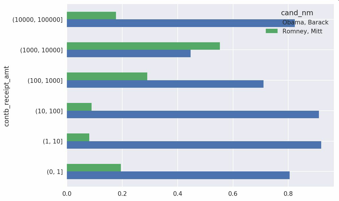
我排除了兩個最大的面元,因為這些不是由個人捐贈的。
還可以對該分析過程做許多的提煉和改進。比如說,可以根據贊助人的姓名和郵編對數據進行聚合,以便找出哪些人進行了多次小額捐款,哪些人又進行了一次或多次大額捐款。我強烈建議你下載這些數據并自己摸索一下。
## 根據州統計贊助信息
根據候選人和州對數據進行聚合是常規操作:
```python
In [220]: grouped = fec_mrbo.groupby(['cand_nm', 'contbr_st'])
In [221]: totals = grouped.contb_receipt_amt.sum().unstack(0).fillna(0)
In [222]: totals = totals[totals.sum(1) > 100000]
In [223]: totals[:10]
Out[223]:
cand_nm Obama, Barack Romney, Mitt
contbr_st
AK 281840.15 86204.24
AL 543123.48 527303.51
AR 359247.28 105556.00
AZ 1506476.98 1888436.23
CA 23824984.24 11237636.60
CO 2132429.49 1506714.12
CT 2068291.26 3499475.45
DC 4373538.80 1025137.50
DE 336669.14 82712.00
FL 7318178.58 8338458.81
```
如果對各行除以總贊助額,就會得到各候選人在各州的總贊助額比例:
```python
In [224]: percent = totals.div(totals.sum(1), axis=0)
In [225]: percent[:10]
Out[225]:
cand_nm Obama, Barack Romney, Mitt
contbr_st
AK 0.765778 0.234222
AL 0.507390 0.492610
AR 0.772902 0.227098
AZ 0.443745 0.556255
CA 0.679498 0.320502
CO 0.585970 0.414030
CT 0.371476 0.628524
DC 0.810113 0.189887
DE 0.802776 0.197224
FL 0.467417 0.532583
```
#14.6 總結
我們已經完成了正文的最后一章。附錄中有一些額外的內容,可能對你有用。
本書第一版出版已經有5年了,Python已經成為了一個流行的、廣泛使用的數據分析語言。你從本書中學到的方法,在相當長的一段時間都是可用的。我希望本書介紹的工具和庫對你的工作有用。
- 利用 Python 進行數據分析 · 第 2 版
- 第 1 章 準備工作
- 第 2 章 Python 語法基礎,IPython 和 Jupyter Notebooks
- 第 3 章 Python 的數據結構、函數和文件
- 第 4 章 NumPy 基礎:數組和矢量計算
- 第 5 章 pandas 入門
- 第 6 章 數據加載、存儲與文件格式
- 第 7 章 數據清洗和準備
- 第 8 章 數據規整:聚合、合并和重塑
- 第 9 章 繪圖和可視化
- 第 10 章 數據聚合與分組運算
- 第 11 章 時間序列
- 第 12 章 pandas 高級應用
- 第 13 章 Python 建模庫介紹
- 第 14 章 數據分析案例
- 附錄 A NumPy 高級應用
- 附錄 B 更多關于 IPython 的內容