**Terry鄧： 這篇文章是我Terry對 普林斯頓 Victor Zhou 有關機器學習“神經網絡”介紹的神文的改進、翻譯 和 重構（重構神經網絡架構）。Victor Zhou的那篇神文是英文的，我先把原文粘貼上來……他的神文雖好，但我 改進更好。所以，大家別忘記回來啊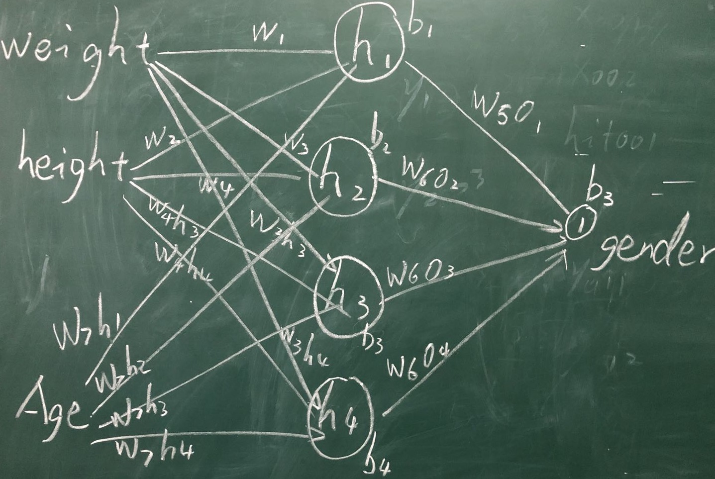！ ## A simple explanation of how they work and how to implement one from scratch in Python. March 3, 2019?|?UPDATED July 24, 2019 Here’s something that might surprise you: **neural networks aren’t that complicated!** The term “neural network” gets used as a buzzword a lot, but in reality they’re often much simpler than people imagine. **This post is intended for complete beginners and assumes ZERO prior knowledge of machine learning**. We’ll understand how neural networks work while implementing one from scratch in Python. Let’s get started! ## 1\. Building Blocks: Neurons First, we have to talk about neurons, the basic unit of a neural network. **A neuron takes inputs, does some math with them, and produces one output**. Here’s what a 2-input neuron looks like:  3 things are happening here. First, each input is multiplied by a weight: x1→x1?w1x\_1 \\rightarrow x\_1 \* w\_1x1?→x1??w1? x2→x2?w2x\_2 \\rightarrow x\_2 \* w\_2x2?→x2??w2? Next, all the weighted inputs are added together with a bias bbb: (x1?w1)+(x2?w2)+b(x\_1 \* w\_1) + (x\_2 \* w\_2) + b(x1??w1?)+(x2??w2?)+b Finally, the sum is passed through an activation function: y\=f(x1?w1+x2?w2+b)y = f(x\_1 \* w\_1 + x\_2 \* w\_2 + b)y\=f(x1??w1?+x2??w2?+b) The activation function is used to turn an unbounded input into an output that has a nice, predictable form. A commonly used activation function is the [sigmoid](https://en.wikipedia.org/wiki/Sigmoid_function) function:  The sigmoid function only outputs numbers in the range (0,1)(0, 1)(0,1). You can think of it as compressing (?∞,+∞)(-\\infty, +\\infty)(?∞,+∞) to (0,1)(0, 1)(0,1) - big negative numbers become ~000, and big positive numbers become ~111. ### A Simple Example Assume we have a 2-input neuron that uses the sigmoid activation function and has the following parameters: w\=\[0,1\]w = \[0, 1\]w\=\[0,1\] b\=4b = 4b\=4 w\=\[0,1\]w = \[0, 1\]w\=\[0,1\] is just a way of writing w1\=0,w2\=1w\_1 = 0, w\_2 = 1w1?\=0,w2?\=1 in vector form. Now, let’s give the neuron an input of x\=\[2,3\]x = \[2, 3\]x\=\[2,3\]. We’ll use the [dot product](https://simple.wikipedia.org/wiki/Dot_product) to write things more concisely: (w?x)+b\=((w1?x1)+(w2?x2))+b\=0?2+1?3+4\=7\\begin{aligned} (w \\cdot x) + b &= ((w\_1 \* x\_1) + (w\_2 \* x\_2)) + b \\\\ &= 0 \* 2 + 1 \* 3 + 4 \\\\ &= 7 \\\\ \\end{aligned}(w?x)+b?\=((w1??x1?)+(w2??x2?))+b\=0?2+1?3+4\=7? y\=f(w?x+b)\=f(7)\=0.999y = f(w \\cdot x + b) = f(7) = \\boxed{0.999}y\=f(w?x+b)\=f(7)\=0.999? The neuron outputs 0.9990.9990.999 given the inputs x\=\[2,3\]x = \[2, 3\]x\=\[2,3\]. That’s it! This process of passing inputs forward to get an output is known as **feedforward**. ### Coding a Neuron Time to implement a neuron! We’ll use [NumPy](https://www.numpy.org/), a popular and powerful computing library for Python, to help us do math: 因為Python的源代碼，幾乎是最靠近人類語言的代碼了……。而且代碼非常清晰…… 從零架構一個 “神經網絡”， 這里的 代碼寫得非常清晰了。 所以，這里直接貼 我 改進的源代碼吧（我 感覺這里代碼比較清晰、注釋也盡量詳盡了）**： ``` import numpy as nump0y001 #這個“import numpy"中的 “numpy系統”是Python的一種開源的數值計算擴展。這種工具可用來存儲和處理大型矩陣，比Python自身的嵌套列表（nested list structure)結構要高效的多（該結構也可以用來表示矩陣（matrix）這里有關Numpy先講這些。……如果您感覺這個numpy成為你的閱讀障礙，那么您可以先跳過……以后咱們再惡補Numpy這部分的知識吧……。 def func_Sigmoid(x): #定義“原傳遞函數”（或稱“sigmoid激活函數”、“激勵函數”、“Sigmoid原函數”……等等、都是它咯……）。 gmoid activation function: f(x) = 1 / (1 + e^(-x)) return 1 / (1 + nump0y001.exp(-x)) def deriv_sigmoid(x): #這是“傳遞函數”的 導函數， 或者稱：“原Sigmoid函數的導函數” # Derivative of func_Sigmoid: f'(x) = f(x) * (1 - f(x)) sigmoidPrimitiveFxFunction = func_Sigmoid(x) return sigmoidPrimitiveFxFunction * (1 - sigmoidPrimitiveFxFunction) def mse_loss(y_true, y_pred): # y_true and y_pred are numpy arrays of the same length. return ((y_true - y_pred) ** 2).mean() #均值函數numpy.mean class OurNeuralNetwork: ''' A neural network with: - 2 inputs - a hidden layer with 2 neurons (h1, h2) - an output layer with 1 neuron (o1) *** DISCLAIMER ***: The code below is intended to be simple and educational, NOT optimal. Real neural net code looks nothing like this. DO NOT use this code. Instead, read/run it to understand how this specific network works. ''' def __init__(self): # Weights self.w1 = nump0y001.random.normal() self.w2 = nump0y001.random.normal() self.w3 = nump0y001.random.normal() self.w3h3 = nump0y001.random.normal() #多出來兩個h(隱含層Cell）第h3（個隱含層Cell細胞） self.w3h4 = nump0y001.random.normal() #多出來兩個H(隱含Cell)第h4 self.w4 = nump0y001.random.normal() self.w4h3 = nump0y001.random.normal() #多出來兩個h(隱含層Cell__命名為h3 self.w4h4 = nump0y001.random.normal() #多出來兩個H(隱含Cell)第h4 self.w5 = nump0y001.random.normal() self.w6 = nump0y001.random.normal() # self.w6b3 = nump0y001.random.normal() self.w6o3 = nump0y001.random.normal() #多出來兩個h(隱含Cell)第O3 self.w6o4 = nump0y001.random.normal() #多出來兩個H(隱含Cell)第O4 #增加一個輸入 x3: Age self.w7h1 = nump0y001.random.normal() self.w7h2 = nump0y001.random.normal() self.w7h3 = nump0y001.random.normal() self.w7h4 = nump0y001.random.normal() # Biases self.b1 = nump0y001.random.normal() self.b2 = nump0y001.random.normal() self.b3 = nump0y001.random.normal() self.b4 = nump0y001.random.normal() def feedforward(self, x): # x is a numpy array with 2 elements. #h1 = func_Sigmoid(self.w1 * x[0] + self.w2 * x[1] + self.b1) h1 = func_Sigmoid(self.w1 * x[0] + self.w2 * x[1] + self.w7h1*x[2]+self.b1) #h2 = func_Sigmoid(self.w3 * x[0] + self.w4 * x[1] + self.b2) h2=func_Sigmoid(self.w3 * x[0] + self.w4 * x[1] + self.w7h2*x[2]+self.b2) #o1 = func_Sigmoid(self.w5 * h1 + self.w6 * h2 + self.b3) h3=func_Sigmoid(self.w3h3 * x[0] + self.w4h3 * x[1] + self.w7h3*x[2]+self.b3) h4=func_Sigmoid(self.w3h4 * x[0] + self.w4h4 * x[1] + self.w7h4*x[2]+self.b4) o1 = func_Sigmoid(self.w5 * h1 + self.w6 * h2 + self.w6o3*h3+ self.w6o4*h4+ self.b3) #self.w6b3*x[3]+self.b3) return o1 def train(self, data, all_y_trues): ''' - data is a (n x 2) numpy array, n = # of samples in the dataset. - all_y_trues is a numpy array with n elements. Elements in all_y_trues correspond to those in data. ''' learn_rate = 0.1 #這里是訓練的 步長，暫時不動用原來默認的。 epochs = 1000 # number of times to loop through the entire dataset for epoch in range(epochs): for x, y_true in zip(data, all_y_trues): # --- Do a feedforward (we'll need these values later) #sum_h1 = self.w1 * x[0] + self.w2 * x[1] + self.b1 sum_h1 = self.w1 * x[0] + self.w2 * x[1] + self.w7h1 * x[2] + self.b1 h1 = func_Sigmoid(sum_h1) sum_h2 = self.w3 * x[0] + self.w4 * x[1] + self.w7h2 * x[2] + self.b2 h2 = func_Sigmoid(sum_h2) sum_h3 = self.w3h3 * x[0] + self.w4h3 * x[1] + self.w7h3*x[2]+self.b2 h3 = func_Sigmoid(sum_h3) sum_h4 = self.w3h3 * x[0] + self.w4h3 * x[1] + self.w7h4 * x[2] + self.b2 h4 = func_Sigmoid(sum_h4) #sum_o1 = self.w5 * h1 + self.w6 * h2 + self.b3 sum_o1 = self.w5 * h1 + self.w6 * h2 + self.w6o3*h3+ h4*self.w6o4+ self.b3 o1 = func_Sigmoid(sum_o1) y_pred = o1 # --- Calculate partial derivatives. # --- Naming: d_L_d_w1 represents "partial L / partial w1" d_L_d_ypred = -2 * (y_true - y_pred) # Neuron o1 d_ypred_d_w5 = h1 * deriv_sigmoid(sum_o1) d_ypred_d_w6 = h2 * deriv_sigmoid(sum_o1) d_ypred_d_w6o3 = h3 * deriv_sigmoid(sum_o1) d_ypred_d_w6o4 = h4 * deriv_sigmoid(sum_o1) d_ypred_d_b3 = deriv_sigmoid(sum_o1) d_ypred_d_h1 = self.w5 * deriv_sigmoid(sum_o1) d_ypred_d_h2 = self.w6 * deriv_sigmoid(sum_o1) d_ypred_d_h3 = self.w6o3 * deriv_sigmoid(sum_o1) d_ypred_d_h4 = self.w6o4 * deriv_sigmoid(sum_o1) # Neuron h1 d_h1_d_w1 = x[0] * deriv_sigmoid(sum_h1) d_h1_d_w2 = x[1] * deriv_sigmoid(sum_h1) d_h1_d_w7=x[2]*deriv_sigmoid(sum_h1) d_h1_d_b1 = deriv_sigmoid(sum_h1) # Neuron h2 d_h2_d_w3 = x[0] * deriv_sigmoid(sum_h2) d_h2_d_w4 = x[1] * deriv_sigmoid(sum_h2) d_h2_d_w7 = x[2] *deriv_sigmoid(sum_h2) d_h2_d_b2 = deriv_sigmoid(sum_h2) # Neuron h3 d_h3_d_w3h3 = x[0] * deriv_sigmoid(sum_h3) d_h3_d_w4h3 = x[1] * deriv_sigmoid(sum_h3) d_h3_d_w7h3 = x[2] *deriv_sigmoid(sum_h3) d_h3_d_b2h3 = deriv_sigmoid(sum_h3) # Neuron h4 d_h4_d_w3h4 = x[0] * deriv_sigmoid(sum_h4) d_h4_d_w4h4 = x[1] * deriv_sigmoid(sum_h4) d_h4_d_w7h4 = x[2] *deriv_sigmoid(sum_h4) d_h4_d_b2h4 = deriv_sigmoid(sum_h4) # --- Update weights and biases # Neuron h1 self.w1 -= learn_rate * d_L_d_ypred * d_ypred_d_h1 * d_h1_d_w1 self.w2 -= learn_rate * d_L_d_ypred * d_ypred_d_h1 * d_h1_d_w2 self.w7h1 -= learn_rate * d_L_d_ypred * d_ypred_d_h1 * d_h1_d_w7 self.b1 -= learn_rate * d_L_d_ypred * d_ypred_d_h1 * d_h1_d_b1 # Neuron h2 self.w3 -= learn_rate * d_L_d_ypred * d_ypred_d_h2 * d_h2_d_w3 self.w4 -= learn_rate * d_L_d_ypred * d_ypred_d_h2 * d_h2_d_w4 self.w7h2 -=learn_rate * d_L_d_ypred * d_ypred_d_h2 * d_h2_d_w7 self.b2 -= learn_rate * d_L_d_ypred * d_ypred_d_h2 * d_h2_d_b2 # Neuron h3 self.w3h3 -= learn_rate * d_L_d_ypred * d_ypred_d_h3 * d_h3_d_w3h3 self.w4h3 -= learn_rate * d_L_d_ypred * d_ypred_d_h3 * d_h3_d_w4h3 self.w7h3 -=learn_rate * d_L_d_ypred * d_ypred_d_h3 * d_h3_d_w7h3 self.b3 -= learn_rate * d_L_d_ypred * d_ypred_d_h3 * d_h3_d_b2h3 # Neuron h4 self.w3h4 -= learn_rate * d_L_d_ypred * d_ypred_d_h4 * d_h4_d_w3h4 self.w4h4 -= learn_rate * d_L_d_ypred * d_ypred_d_h4 * d_h4_d_w4h4 self.w7h4 -=learn_rate * d_L_d_ypred * d_ypred_d_h4 * d_h4_d_w7h4 self.b4 -= learn_rate * d_L_d_ypred * d_ypred_d_h4 * d_h4_d_b2h4 # Neuron o1 self.w5 -= learn_rate * d_L_d_ypred * d_ypred_d_w5 self.w6 -= learn_rate * d_L_d_ypred * d_ypred_d_w6 self.w6o3 -= learn_rate * d_L_d_ypred * d_ypred_d_w6o3 self.w6o4 -= learn_rate * d_L_d_ypred * d_ypred_d_w6o4 self.b3 -= learn_rate * d_L_d_ypred * d_ypred_d_b3 # --- Calculate total loss at the end of each epoch if epoch % 10 == 0: y_preds = nump0y001.apply_along_axis(self.feedforward, 1, data) loss = mse_loss(all_y_trues, y_preds) print("Epoch %d loss: %.3f" % (epoch, loss)) # Define dataset #原來輸入只有： x1:體重, x2身高 #我這里 增加 第3個 輸入： x3: 即年齡 ''' /*data = nump0y001.array([ [-2, -1], # Alice [25, 6], # Bob [17, 4], # Charlie [-15, -6], # Diana ])*/ ''' #我這里 增加 第3個 輸入： x3: 即年齡 data = nump0y001.array([ [-2, -1 , 15], # Alice [25, 6, 55], # Bob [17, 4, 65], # Charlie [-15, -6, 19], # Diana ]) all_y_trues = nump0y001.array([ 1, # Alice 0, # Bob 0, # Charlie 1, # Diana ]) # Train our neural network!這里是 Trainning訓練函數 調用 network = OurNeuralNetwork() network.train(data, all_y_trues) # Make some predictions #emily = nump0y001.array([-7, -3]) # 128 pounds, 63 inches #= nump0y001.array([-7, -3, 19]) # 這里 也 增加了 第三個 參數值：即年齡數，如：19(Age) emily = nump0y001.array([-7, -3, 19]) # 128 pounds, 63 inches, Ages:19 #frank = nump0y001.array([20, 2]) # 155 pounds, 68 inches frank = nump0y001.array([20, 2, 60]) # 155 pounds, 68 inches, Age:60 print("Emily: %.3f" % network.feedforward(emily)) # 0.951 - F print("Frank: %.3f" % network.feedforward(frank)) # 0.039 - M #鏈接：https://www. ``` 運行結果： ``` aw3@aw3-ThinkPad-X220-Tablet:~/ann01numpy01$ python3 03ann02zhou02numpy03.py Epoch 0 loss: 0.318 Epoch 10 loss: 0.112 Epoch 20 loss: 0.057 Epoch 30 loss: 0.042 Epoch 40 loss: 0.035 Epoch 50 loss: 0.031 Epoch 60 loss: 0.028 Epoch 70 loss: 0.025 Epoch 80 loss: 0.023 Epoch 90 loss: 0.021 Epoch 100 loss: 0.019 Epoch 110 loss: 0.018 Epoch 120 loss: 0.017 Epoch 130 loss: 0.016 Epoch 140 loss: 0.015 Epoch 150 loss: 0.014 Epoch 160 loss: 0.014 Epoch 170 loss: 0.013 Epoch 180 loss: 0.012 Epoch 190 loss: 0.012 Epoch 200 loss: 0.011 Epoch 210 loss: 0.011 Epoch 220 loss: 0.010 Epoch 230 loss: 0.010 Epoch 240 loss: 0.010 Epoch 250 loss: 0.009 Epoch 260 loss: 0.009 Epoch 270 loss: 0.009 Epoch 280 loss: 0.008 Epoch 290 loss: 0.008 Epoch 300 loss: 0.008 Epoch 310 loss: 0.008 Epoch 320 loss: 0.007 Epoch 330 loss: 0.007 Epoch 340 loss: 0.007 Epoch 350 loss: 0.007 Epoch 360 loss: 0.007 Epoch 370 loss: 0.006 Epoch 380 loss: 0.006 Epoch 390 loss: 0.006 Epoch 400 loss: 0.006 Epoch 410 loss: 0.006 Epoch 420 loss: 0.006 Epoch 430 loss: 0.006 Epoch 440 loss: 0.005 Epoch 450 loss: 0.005 Epoch 460 loss: 0.005 Epoch 470 loss: 0.005 Epoch 480 loss: 0.005 Epoch 490 loss: 0.005 Epoch 500 loss: 0.005 Epoch 510 loss: 0.005 Epoch 520 loss: 0.005 Epoch 530 loss: 0.004 Epoch 540 loss: 0.004 Epoch 550 loss: 0.004 Epoch 560 loss: 0.004 Epoch 570 loss: 0.004 Epoch 580 loss: 0.004 Epoch 590 loss: 0.004 Epoch 600 loss: 0.004 Epoch 610 loss: 0.004 Epoch 620 loss: 0.004 Epoch 630 loss: 0.004 Epoch 640 loss: 0.004 Epoch 650 loss: 0.004 Epoch 660 loss: 0.004 Epoch 670 loss: 0.004 Epoch 680 loss: 0.004 Epoch 690 loss: 0.003 Epoch 700 loss: 0.003 Epoch 710 loss: 0.003 Epoch 720 loss: 0.003 Epoch 730 loss: 0.003 Epoch 740 loss: 0.003 Epoch 750 loss: 0.003 Epoch 760 loss: 0.003 Epoch 770 loss: 0.003 Epoch 780 loss: 0.003 Epoch 790 loss: 0.003 Epoch 800 loss: 0.003 Epoch 810 loss: 0.003 Epoch 820 loss: 0.003 Epoch 830 loss: 0.003 Epoch 840 loss: 0.003 Epoch 850 loss: 0.003 Epoch 860 loss: 0.003 Epoch 870 loss: 0.003 Epoch 880 loss: 0.003 Epoch 890 loss: 0.003 Epoch 900 loss: 0.003 Epoch 910 loss: 0.003 Epoch 920 loss: 0.003 Epoch 930 loss: 0.003 Epoch 940 loss: 0.003 Epoch 950 loss: 0.003 Epoch 960 loss: 0.002 Epoch 970 loss: 0.002 Epoch 980 loss: 0.002 Epoch 990 loss: 0.002 Emily: 0.948 Frank: 0.045 ``` 請注意，結果收斂得不錯 Emily的 得分： 0.948 性別得分 接近 女性（標準得分）：即1 Frank的 得分： 0.045 性別得分 接近 男性的 標準得分： 0 **所謂 改進， 我 增加 了 網絡的 復雜度： 1、增加了 一個 輸入 X[2] 2、 增加 了 隱含層 的 兩個 細胞(Cells) 即 H3 和 H4 這樣，在 原有 網絡 的 基礎上， 咱們 就 可以 達到， 改進 和重新 架構 “神經網絡”的 效果和功能 了： 新的“神經網絡”網絡架構如下**：  下面是： 普林斯頓 Victor Zhou有關機器學習“神經網絡”介紹的神文雖好，但我 改進更好。所以，大家別忘記回來啊！ [普林斯頓Victor Zhou的博客介紹神文鏈接](https://victorzhou.com/blog/intro-to-neural-networks/)