九、啟動并運行 TensorFlow · Sklearn 與 TensorFlow 機器學習實用指南

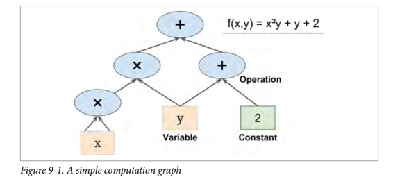
# 九、啟動并運行 TensorFlow > 譯者：[@akonwang](https://github.com/wangxupeng)、[@WilsonQu](https://github.com/WilsonQu) > > 校對者：[@Lisanaaa](https://github.com/Lisanaaa)、[@飛龍](https://github.com/wizardforcel)、[@YuWang](https://github.com/bigeyex) TensorFlow 是一款用于數值計算的強大的開源軟件庫，特別適用于大規模機器學習的微調。它的基本原理很簡單：首先在 Python 中定義要執行的計算圖（例如圖 9-1），然后 TensorFlow 使用該圖并使用優化的 C++ 代碼高效運行該圖。 ![](https://img.kancloud.cn/9b/95/9b95cd2d6261b0726d19494d963c65ab_566x268.png) 最重要的是，Tensorflow 可以將圖分解為多個塊并在多個 CPU 或 GPU 上并行運行（如圖 9-2 所示）。 TensorFlow 還支持分布式計算，因此您可以在數百臺服務器上分割計算，從而在合理的時間內在龐大的訓練集上訓練龐大的神經網絡（請參閱第 12 章）。 TensorFlow 可以訓練一個擁有數百萬個參數的網絡，訓練集由數十億個具有數百萬個特征的實例組成。這應該不會讓您吃驚，因為 TensorFlow 是由Google 大腦團隊開發的，它支持谷歌的大量服務，例如 Google Cloud Speech，Google Photos 和 Google Search。 ![](https://img.kancloud.cn/7d/8b/7d8ba1c4ace2aa4cd1094e8d085209c8_566x380.png) 當 TensorFlow 于 2015 年 11 月開放源代碼時，已有許多深度學習的流行開源庫（表 9-1 列出了一些），公平地說，大部分 TensorFlow 的功能已經存在于一個庫或另一個庫中。盡管如此，TensorFlow 的整潔設計，可擴展性，靈活性和出色的文檔（更不用說谷歌的名字）迅速將其推向了榜首。簡而言之，TensorFlow 的設計靈活性，可擴展性和生產就緒性，現有框架可以說只有其中三種可用。這里有一些 TensorFlow 的亮點： - 它不僅在 Windows，Linux 和 MacOS 上運行，而且在移動設備上運行，包括 iOS 和 Android。它提供了一個非常簡單的 Python API，名為 TF.Learn2（`tensorflow.con trib.learn`），與 Scikit-Learn 兼容。正如你將會看到的，你可以用幾行代碼來訓練不同類型的神經網絡。之前是一個名為 Scikit Flow（或 Skow）的獨立項目。 - 它還提供了另一個簡單的稱為 TF-slim（`tensorflow.contrib.slim`）的 API 來簡化構建，訓練和求出神經網絡。 - 其他幾個高級 API 已經在 TensorFlow 之上獨立構建，如 **Keras** 或 **Pretty Tensor**。 - 它的主要 Python API 提供了更多的靈活性（以更高復雜度為代價）來創建各種計算，包括任何你能想到的神經網絡結構。 - 它包括許多 ML 操作的高效 C ++ 實現，特別是構建神經網絡所需的 C++ 實現。還有一個 C++ API 來定義您自己的高性能操作。 - 它提供了幾個高級優化節點來搜索最小化損失函數的參數。由于 TensorFlow 自動處理計算您定義的函數的梯度，因此這些非常易于使用。這稱為自動分解（或`autodi`）。 - 它還附帶一個名為 TensorBoard 的強大可視化工具，可讓您瀏覽計算圖表，查看學習曲線等。 - Google 還推出了云服務來運行 TensorFlow 表。 - 最后，它擁有一支充滿熱情和樂于助人的開發團隊，以及一個不斷成長的社區，致力于改善它。它是 GitHub 上最受歡迎的開源項目之一，并且越來越多的優秀項目正在構建之上（例如，查看 <https://www.tensorflow.org/> 或 <https://github.com/jtoy/awesome-tensorflow>）。要問技術問題，您應該使用 <http://stackoverflow.com/> 并用`tensorflow`標記您的問題。您可以通過 GitHub 提交錯誤和功能請求。有關一般討論，請加入 **Google 小組**。 ![](https://img.kancloud.cn/db/cd/dbcd0c08a1cd16c34732d0a05e89d4fe_566x230.png) 在本章中，我們將介紹 TensorFlow 的基礎知識，從安裝到創建，運行，保存和可視化簡單的計算圖。在構建第一個神經網絡之前掌握這些基礎知識很重要（我們將在下一章中介紹）。 ## 安裝讓我們開始吧！假設您按照第 2 章中的安裝說明安裝了 Jupyter 和 Scikit-Learn，您可以簡單地使用`pip`來安裝 TensorFlow。如果你使用`virtualenv`創建了一個獨立的環境，你首先需要激活它： <pre><code> $ cd $ML_PATH #Your ML working directory(e.g., $HOME/ml) $ source env/bin/activate </code></pre> 下一步，安裝 Tensorflow。 ``` $ pip3 install --upgrade tensorflow ``` 對于 GPU 支持，你需要安裝`tensorflow-gpu`而不是`tensorflow`。具體請參見 12 章內容。為了測試您的安裝，請輸入一下命令。其輸出應該是您安裝的 Tensorflow 的版本號。 ``` $ python -c 'import tensorflow; print(tensorflow.__version__)' 1.0.0 ``` ## 創造第一個圖譜，然后運行它 ```python import?tensorflow?as?tf?? x?=?tf.Variable(3,?name="x")?? y?=?tf.Variable(4,?name="y")?? f?=?x*x*y?+?y?+?2?? ``` 這就是它的一切！最重要的是要知道這個代碼實際上并不執行任何計算，即使它看起來像(尤其是最后一行）。它只是創建一個計算圖譜。事實上，變量都沒有初始化.要求出此圖，您需要打開一個 TensorFlow 會話并使用它初始化變量并求出`f`。TensorFlow 會話負責處理在諸如 CPU 和 GPU 之類的設備上的操作并運行它們，并且它保留所有變量值。以下代碼創建一個會話，初始化變量，并求出`f`，然后關閉會話（釋放資源）： ```python #?way1?? sess?=?tf.Session()?? sess.run(x.initializer)?? sess.run(y.initializer)?? result?=?sess.run(f)?? ?? print(result)?? sess.close()?? ``` 不得不每次重復sess.run() 有點麻煩，但幸運的是有一個更好的方法： ```python # way2?? with?tf.Session()?as?sess:?? ????x.initializer.run()?? ????y.initializer.run()?? ????result?=?f.eval()?? print(result)? ``` 在`with`塊中，會話被設置為默認會話。調用`x.initializer.run()`等效于調用`tf.get_default_session().run(x.initial)`，`f.eval()`等效于調用`tf.get_default_session().run(f)`。這使得代碼更容易閱讀。此外，會話在塊的末尾自動關閉。你可以使用`global_variables_initializer()` 函數，而不是手動初始化每個變量。請注意，它實際上沒有立即執行初始化，而是在圖譜中創建一個當程序運行時所有變量都會初始化的節點： ```python # way3?? init?=?tf.global_variables_initializer()?? with?tf.Session()?as?sess:?? ????init.run()?? ????result?=?f.eval()?? ? print(result)?? ``` 在 Jupyter 內部或在 Python shell 中，您可能更喜歡創建一個`InteractiveSession`。與常規會話的唯一區別是，當創建`InteractiveSession`時，它將自動將其自身設置為默認會話，因此您不需要使用模塊（但是您需要在完成后手動關閉會話）： ```python # way4?? init?=?tf.global_variables_initializer()?? sess?=?tf.InteractiveSession()?? init.run()?? result?=?f.eval()?? print(result)?? sess.close()?? ``` TensorFlow 程序通常分為兩部分：第一部分構建計算圖譜（這稱為構造階段），第二部分運行它（這是執行階段）。建設階段通常構建一個表示 ML 模型的計算圖譜,然后對其進行訓練,計算。執行階段通常運行循環，重復地求出訓練步驟（例如，每個小批次），逐漸改進模型參數。? ## 管理圖譜您創建的任何節點都會自動添加到默認圖形中： ```python >>>?x1?=?tf.Variable(1)?? >>>?x1.graph?is?tf.get_default_graph()?? True?? ``` 在大多數情況下，這是很好的，但有時您可能需要管理多個獨立圖形。您可以通過創建一個新的圖形并暫時將其設置為一個塊中的默認圖形，如下所示： ```python >>>?graph?=?tf.Graph()?? >>>?with?graph.as_default():?? ...?x2?=?tf.Variable(2)?? ...?? >>>?x2.graph?is?graph?? True?? >>>?x2.graph?is?tf.get_default_graph()?? False?? ``` 在 Jupyter（或 Python shell）中，通常在實驗時多次運行相同的命令。因此，您可能會收到包含許多重復節點的默認圖形。一個解決方案是重新啟動 Jupyter 內核（或 Python shell），但是一個更方便的解決方案是通過運行`tf.reset_default_graph()`來重置默認圖。 ## 節點值的生命周期求出節點時，TensorFlow 會自動確定所依賴的節點集，并首先求出這些節點。例如，考慮以下代碼： ```python #?w?=?tf.constant(3)?? #?x?=?w?+?2?? #?y?=?x?+?5?? #?z?=?x?*?3?? ?? #?with?tf.Session()?as?sess:?? #?????print(y.eval())?? #?????print(z.eval())?? ``` 首先，這個代碼定義了一個非常簡單的圖。然后，它啟動一個會話并運行圖來求出`y`：TensorFlow 自動檢測到`y`取決于`x`，它取決于`w`，所以它首先求出`w`，然后`x`，然后`y`，并返回`y`的值。最后，代碼運行圖來求出`z`。同樣，TensorFlow 檢測到它必須首先求出`w`和`x`。重要的是要注意，它不會復用以前的w和x的求出結果。簡而言之，前面的代碼求出`w`和`x`兩次。所有節點值都在圖運行之間刪除，除了變量值，由會話跨圖形運行維護（隊列和讀者也保持一些狀態）。變量在其初始化程序運行時啟動其生命周期，并且在會話關閉時結束。如果要有效地求出`y`和`z`，而不像之前的代碼那樣求出`w`和`x`兩次，那么您必須要求 TensorFlow 在一個圖形運行中求出`y`和`z`，如下面的代碼所示： ```python #?with?tf.Session()?as?sess:?? #?????y_val,?z_val?=?sess.run([y,?z])?? #?????print(y_val)?#?10?? #?????print(z_val)?#?15?? ``` 在單進程 TensorFlow 中，多個會話不共享任何狀態，即使它們復用同一個圖（每個會話都有自己的每個變量的副本）。在分布式 TensorFlow 中，變量狀態存儲在服務器上，而不是在會話中，因此多個會話可以共享相同的變量。 ## Linear Regression with TensorFlow TensorFlow 操作（也簡稱為 ops）可以采用任意數量的輸入并產生任意數量的輸出。例如，加法運算和乘法運算都需要兩個輸入并產生一個輸出。常量和變量不輸入（它們被稱為源操作）。輸入和輸出是稱為張量的多維數組（因此稱為“tensor flow”）。就像 NumPy 數組一樣，張量具有類型和形狀。實際上，在 Python API 中，張量簡單地由 NumPy`ndarray`表示。它們通常包含浮點數，但您也可以使用它們來傳送字符串（任意字節數組）。迄今為止的示例，張量只包含單個標量值，但是當然可以對任何形狀的數組執行計算。例如，以下代碼操作二維數組來對加利福尼亞房屋數據集進行線性回歸（在第 2 章中介紹）。它從獲取數據集開始；之后它會向所有訓練實例添加一個額外的偏置輸入特征（`x0 = 1`）（它使用 NumPy 進行，因此立即運行）；之后它創建兩個 TensorFlow 常量節點`X`和`y`來保存該數據和目標，并且它使用 TensorFlow 提供的一些矩陣運算來定義`theta`。這些矩陣函數`transpose()`，`matmul()`和`matrix_inverse()`是不言自明的，但是像往常一樣，它們不會立即執行任何計算；相反，它們會在圖形中創建在運行圖形時執行它們的節點。您可以認識到`θ`的定義對應于方程 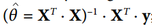![](https://img.kancloud.cn/8b/14/8b14c73b2bd9ccfd22313bb1e4fd92a4_222x42.png)。最后，代碼創建一個`session`并使用它來求出`theta`。 ```python import?numpy?as?np?? from?sklearn.datasets?import?fetch_california_housing?? housing?=?fetch_california_housing()?? m,?n?=?housing.data.shape?? #np.c_按colunm來組合array?? housing_data_plus_bias?=?np.c_[np.ones((m,?1)),?housing.data]?? ?? X?=?tf.constant(housing_data_plus_bias,?dtype=tf.float32,?name="X")?? y?=?tf.constant(housing.target.reshape(-1,?1),?dtype=tf.float32,?name="y")?? XT =?tf.transpose(X)?? theta?=?tf.matmul(tf.matmul(tf.matrix_inverse(tf.matmul(XT,?X)),?XT),?y)?? with?tf.Session()?as?sess:?? ????theta_value?=?theta.eval()?? print(theta_value)?? ``` 如果您有一個 GPU 的話，上述代碼相較于直接使用 NumPy 計算正態方程式的主要優點是 TensorFlow 會自動運行在您的 GPU 上（如果您安裝了支持 GPU 的 TensorFlow，則 TensorFlow 將自動運行在 GPU 上，請參閱第 12 章了解更多詳細信息）。其實這里就是用最小二乘法算`θ` [http://blog.csdn.net/akon_wang_hkbu/article/details/77503725](http://blog.csdn.net/akon_wang_hkbu/article/details/77503725) ## 實現梯度下降讓我們嘗試使用批量梯度下降（在第 4 章中介紹），而不是普通方程。首先，我們將通過手動計算梯度來實現，然后我們將使用 TensorFlow 的自動擴展功能來使 TensorFlow 自動計算梯度，最后我們將使用幾個 TensorFlow 的優化器。當使用梯度下降時，請記住，首先要對輸入特征向量進行歸一化，否則訓練可能要慢得多。您可以使用 TensorFlow，NumPy，Scikit-Learn 的`StandardScaler`或您喜歡的任何其他解決方案。以下代碼假定此規范化已經完成。 ## 手動計算漸變以下代碼應該是相當不言自明的，除了幾個新元素： * `random_uniform()`函數在圖形中創建一個節點，它將生成包含隨機值的張量，給定其形狀和值作用域，就像 NumPy 的`rand()`函數一樣。 * `assign()`函數創建一個為變量分配新值的節點。在這種情況下，它實現了批次梯度下降步驟 ![\theta(next step)= \theta - \eta \nabla_{\theta}MSE(\theta)](https://img.kancloud.cn/30/fc/30fc12ab6ff64e3c9ea62c88bc73a0ab_245x18.gif)。 * 主循環一次又一次（共`n_epochs`次）執行訓練步驟，每 100 次迭代都打印出當前均方誤差（MSE）。你應該看到 MSE 在每次迭代中都會下降。 ```python housing?=?fetch_california_housing()?? m,?n?=?housing.data.shape?? m,?n?=?housing.data.shape?? #np.c_按colunm來組合array?? housing_data_plus_bias?=?np.c_[np.ones((m,?1)),?housing.data]?? scaled_housing_data_plus_bias?=?scale(housing_data_plus_bias)?? n_epochs?=?1000?? learning_rate?=?0.01?? X?=?tf.constant(scaled_housing_data_plus_bias,?dtype=tf.float32,?name="X")?? y?=?tf.constant(housing.target.reshape(-1,?1),?dtype=tf.float32,?name="y")?? theta?=?tf.Variable(tf.random_uniform([n?+?1,?1],?-1.0,?1.0),?name="theta")?? y_pred?=?tf.matmul(X,?theta,?name="predictions")?? error?=?y_pred?-?y?? mse?=?tf.reduce_mean(tf.square(error),?name="mse")?? gradients?=?2/m?*?tf.matmul(tf.transpose(X),?error)?? training_op?=?tf.assign(theta,?theta?-?learning_rate?*?gradients)?? init?=?tf.global_variables_initializer()?? with?tf.Session()?as?sess:?? ????sess.run(init)?? ????for?epoch?in?range(n_epochs):?? ????????if?epoch?%?100?==?0:?? ????????????print("Epoch",?epoch,?"MSE?=",?mse.eval())?? ????????sess.run(training_op)?? ????best_theta?=?theta.eval()?? ``` ## Using autodi? 前面的代碼工作正常，但它需要從代價函數（MSE）中利用數學公式推導梯度。在線性回歸的情況下，這是相當容易的，但是如果你必須用深層神經網絡來做這個事情，你會感到頭痛：這將是乏味和容易出錯的。您可以使用符號求導來為您自動找到偏導數的方程式，但結果代碼不一定非常有效。為了理解為什么，考慮函數`f(x) = exp(exp(exp(x)))`。如果你知道微積分，你可以計算出它的導數`f'(x) = exp(x) * exp(exp(x)) * exp(exp(exp(x)))`。如果您按照普通的計算方式分別去寫`f(x)`和`f'(x)`，您的代碼將不會如此有效。一個更有效的解決方案是寫一個首先計算`exp(x)`，然后`exp(exp(x))`，然后`exp(exp(exp(x)))`的函數，并返回所有三個。這直接給你（第三項）`f(x)`，如果你需要求導，你可以把這三個子式相乘，你就完成了。通過傳統的方法，您不得不將`exp`函數調用 9 次來計算`f(x)`和`f'(x)`。使用這種方法，你只需要調用它三次。當您的功能由某些任意代碼定義時，它會變得更糟。你能找到方程（或代碼）來計算以下函數的偏導數嗎？提示：不要嘗試。 ```python def?my_func(a,?b):?? ????z?=?0?? ????for?i?in?range(100):?? ???? z?=?a?*?np.cos(z?+?i)?+?z?*?np.sin(b?-?i)?? ????return?z?? ``` 幸運的是，TensorFlow 的自動計算梯度功能可以計算這個公式：它可以自動高效地為您計算梯度。只需用以下面這行代碼替換上一節中代碼的`gradients = ...`行，代碼將繼續工作正常： ```python gradients?=?tf.gradients(mse,?[theta])[0]?? ``` `gradients()`函數使用一個`op`（在這種情況下是MSE）和一個變量列表（在這種情況下只是`theta`），它創建一個`ops`列表（每個變量一個）來計算`op`的梯度變量。因此，梯度節點將計算 MSE 相對于`theta`的梯度向量。自動計算梯度有四種主要方法。它們總結在表 9-2 中。 TensorFlow 使用反向模式，這是完美的（高效和準確），當有很多輸入和少量的輸出，如通常在神經網絡的情況。它只需要通過 ![n_{outputs} + 1](https://img.kancloud.cn/a1/ab/a1ab314fc4efa6bf80a72dfd4c9efb96_85x18.gif) 次圖遍歷即可計算所有輸出的偏導數。 ![](/images/chapter_9/20171030144740842.jpg) ## 使用優化器所以 TensorFlow 為您計算梯度。但它還有更好的方法：它還提供了一些可以直接使用的優化器，包括梯度下降優化器。您可以使用以下代碼簡單地替換以前的`gradients = ...`和`training_op = ...`行，并且一切都將正常工作： ```python optimizer?=?tf.train.GradientDescentOptimizer(learning_rate=learning_rate)?? training_op?=?optimizer.minimize(mse)?? ``` 如果要使用其他類型的優化器，則只需要更改一行。例如，您可以通過定義優化器來使用動量優化器（通常會比漸變收斂的收斂速度快得多；參見第 11 章） ```python optimizer?=?tf.train.MomentumOptimizer(learning_rate=learning_rate,?momentum=0.9)?? ``` ## 將數據提供給訓練算法我們嘗試修改以前的代碼來實現小批量梯度下降（Mini-batch Gradient Descent）。為此，我們需要一種在每次迭代時用下一個小批量替換`X`和`Y`的方法。最簡單的方法是使用占位符（placeholder）節點。這些節點是特別的，因為它們實際上并不執行任何計算，只是輸出您在運行時輸出的數據。它們通常用于在訓練期間將訓練數據傳遞給 TensorFlow。如果在運行時沒有為占位符指定值，則會收到異常。要創建占位符節點，您必須調用`placeholder()`函數并指定輸出張量的數據類型。或者，您還可以指定其形狀，如果要強制執行。如果指定維度為`None`，則表示“任何大小”。例如，以下代碼創建一個占位符節點`A`，還有一個節點`B = A + 5`。當我們求出`B`時，我們將一個`feed_dict`傳遞給`eval()`方法并指定`A`的值。注意，`A`必須具有 2 級（即它必須是二維的），并且必須有三列（否則引發異常），但它可以有任意數量的行。 ```python >>>?A?=?tf.placeholder(tf.float32,?shape=(None,?3))?? >>>?B?=?A?+?5?? >>>?with?tf.Session()?as?sess:?? ...?B_val_1?=?B.eval(feed_dict={A:?[[1,?2,?3]]})?? ...?B_val_2?=?B.eval(feed_dict={A:?[[4,?5,?6],?[7,?8,?9]]})?? ...?? >>>?print(B_val_1)?? [[?6.?7.?8.]]?? >>>?print(B_val_2)?? [[?9.?10.?11.]?? [?12.?13.?14.]]?? ``` 您實際上可以提供任何操作的輸出，而不僅僅是占位符。在這種情況下，TensorFlow 不會嘗試求出這些操作；它使用您提供的值。要實現小批量漸變下降，我們只需稍微調整現有的代碼。首先更改`X`和`Y`的定義，使其定義為占位符節點： ```python X?=?tf.placeholder(tf.float32,?shape=(None,?n?+?1),?name="X")?? y?=?tf.placeholder(tf.float32,?shape=(None,?1),?name="y")?? ``` 然后定義批量大小并計算總批次數： ```python batch_size?=?100?? n_batches?=?int(np.ceil(m?/?batch_size))?? ``` 最后，在執行階段，逐個獲取小批量，然后在求出依賴于`X`和`y`的值的任何一個節點時，通過`feed_dict`提供`X`和`y`的值。 ```python def fetch_batch(epoch, batch_index, batch_size): [...] # load the data from disk return X_batch, y_batch with tf.Session() as sess: sess.run(init) for epoch in range(n_epochs): for batch_index in range(n_batches): X_batch, y_batch = fetch_batch(epoch, batch_index, batch_size) sess.run(training_op, feed_dict={X: X_batch, y: y_batch}) best_theta = theta.eval() ``` 在求出theta時，我們不需要傳遞X和y的值，因為它不依賴于它們。 ## MINI-BATCH 完整代碼 ```python import?numpy?as?np?? from?sklearn.datasets?import?fetch_california_housing?? import?tensorflow?as?tf?? from?sklearn.preprocessing?import?StandardScaler?? ?? housing?=?fetch_california_housing()?? m,?n?=?housing.data.shape?? print("數據集:{}行,{}列".format(m,n))?? housing_data_plus_bias?=?np.c_[np.ones((m,?1)),?housing.data]?? scaler?=?StandardScaler()?? scaled_housing_data?=?scaler.fit_transform(housing.data)?? scaled_housing_data_plus_bias?=?np.c_[np.ones((m,?1)),?scaled_housing_data]?? ?? n_epochs?=?1000?? learning_rate?=?0.01?? ?? X?=?tf.placeholder(tf.float32,?shape=(None,?n?+?1),?name="X")?? y?=?tf.placeholder(tf.float32,?shape=(None,?1),?name="y")?? theta?=?tf.Variable(tf.random_uniform([n?+?1,?1],?-1.0,?1.0,?seed=42),?name="theta")?? y_pred?=?tf.matmul(X,?theta,?name="predictions")?? error?=?y_pred?-?y?? mse?=?tf.reduce_mean(tf.square(error),?name="mse")?? optimizer?=?tf.train.GradientDescentOptimizer(learning_rate=learning_rate)?? training_op?=?optimizer.minimize(mse)?? ?? init?=?tf.global_variables_initializer()?? ?? n_epochs?=?10?? batch_size?=?100?? n_batches?=?int(np.ceil(m?/?batch_size))?# ceil() 方法返回 x 的值上限?-?不小于 x 的最小整數。?? ?? def?fetch_batch(epoch,?batch_index,?batch_size):?? ????know?=?np.random.seed(epoch?*?n_batches?+?batch_index)??#?not?shown?in?the?book?? ????print("我是know:",know)?? ????indices?=?np.random.randint(m,?size=batch_size)??#?not?shown?? ????X_batch?=?scaled_housing_data_plus_bias[indices]?#?not?shown?? ????y_batch?=?housing.target.reshape(-1,?1)[indices]?#?not?shown?? ????return?X_batch,?y_batch?? ?? with?tf.Session()?as?sess:?? ????sess.run(init)?? ?? ????for?epoch?in?range(n_epochs):?? ????????for?batch_index?in?range(n_batches):?? ????????????X_batch,?y_batch?=?fetch_batch(epoch,?batch_index,?batch_size)?? ????????????sess.run(training_op,?feed_dict={X:?X_batch,?y:?y_batch})?? ?? ????best_theta?=?theta.eval()?? ?? print(best_theta)?? ``` ## 保存和恢復模型一旦你訓練了你的模型，你應該把它的參數保存到磁盤，所以你可以隨時隨地回到它，在另一個程序中使用它，與其他模型比較，等等。此外，您可能希望在訓練期間定期保存檢查點，以便如果您的計算機在訓練過程中崩潰，您可以從上次檢查點繼續進行，而不是從頭開始。 TensorFlow 可以輕松保存和恢復模型。只需在構造階段結束（創建所有變量節點之后）創建一個保存節點; 那么在執行階段，只要你想保存模型，只要調用它的`save()`方法: ```python [...] theta = tf.Variable(tf.random_uniform([n + 1, 1], -1.0, 1.0), name="theta") [...] init = tf.global_variables_initializer() saver = tf.train.Saver() with tf.Session() as sess: sess.run(init) for epoch in range(n_epochs): if epoch % 100 == 0: # checkpoint every 100 epochs save_path = saver.save(sess, "/tmp/my_model.ckpt") sess.run(training_op) best_theta = theta.eval() save_path = saver.save(sess, "/tmp/my_model_final.ckpt") ``` 恢復模型同樣容易：在構建階段結束時創建一個保存器，就像之前一樣，但是在執行階段的開始，而不是使用`init`節點初始化變量，你可以調用`restore()`方法的保存器對象： ```python with tf.Session() as sess: saver.restore(sess, "/tmp/my_model_final.ckpt") [...] ``` 默認情況下，保存器將以自己的名稱保存并還原所有變量，但如果需要更多控制，則可以指定要保存或還原的變量以及要使用的名稱。例如，以下保存器將僅保存或恢復`theta`變量，它的鍵名稱是`weights`： ``` saver = tf.train.Saver({"weights": theta}) ``` 完整代碼 ```python import numpy as np from sklearn.datasets import fetch_california_housing import tensorflow as tf from sklearn.preprocessing import StandardScaler housing = fetch_california_housing() m, n = housing.data.shape print("數據集:{}行,{}列".format(m,n)) housing_data_plus_bias = np.c_[np.ones((m, 1)), housing.data] scaler = StandardScaler() scaled_housing_data = scaler.fit_transform(housing.data) scaled_housing_data_plus_bias = np.c_[np.ones((m, 1)), scaled_housing_data] n_epochs = 1000 # not shown in the book learning_rate = 0.01 # not shown X = tf.constant(scaled_housing_data_plus_bias, dtype=tf.float32, name="X") # not shown y = tf.constant(housing.target.reshape(-1, 1), dtype=tf.float32, name="y") # not shown theta = tf.Variable(tf.random_uniform([n + 1, 1], -1.0, 1.0, seed=42), name="theta") y_pred = tf.matmul(X, theta, name="predictions") # not shown error = y_pred - y # not shown mse = tf.reduce_mean(tf.square(error), name="mse") # not shown optimizer = tf.train.GradientDescentOptimizer(learning_rate=learning_rate) # not shown training_op = optimizer.minimize(mse) # not shown init = tf.global_variables_initializer() saver = tf.train.Saver() with tf.Session() as sess: sess.run(init) for epoch in range(n_epochs): if epoch % 100 == 0: print("Epoch", epoch, "MSE =", mse.eval()) # not shown save_path = saver.save(sess, "/tmp/my_model.ckpt") sess.run(training_op) best_theta = theta.eval() save_path = saver.save(sess, "/tmp/my_model_final.ckpt") #找到tmp文件夾就找到文件了 ``` 使用 TensorBoard 展現圖形和訓練曲線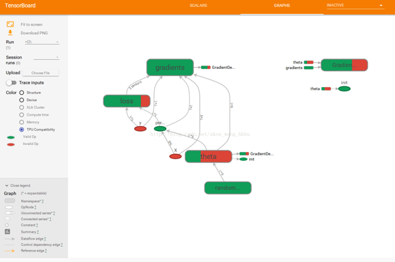所以現在我們有一個使用小批量梯度下降訓練線性回歸模型的計算圖譜，我們正在定期保存檢查點。聽起來很復雜，不是嗎？然而，我們仍然依靠`print()`函數可視化訓練過程中的進度。有一個更好的方法：進入 TensorBoard。如果您提供一些訓練統計信息，它將在您的網絡瀏覽器中顯示這些統計信息的良好交互式可視化（例如學習曲線）。您還可以提供圖形的定義，它將為您提供一個很好的界面來瀏覽它。這對于識別圖中的錯誤，找到瓶頸等是非常有用的。第一步是調整程序，以便將圖形定義和一些訓練統計信息（例如，`training_error`（MSE））寫入 TensorBoard 將讀取的日志目錄。您每次運行程序時都需要使用不同的日志目錄，否則 TensorBoard 將會合并來自不同運行的統計信息，這將會混亂可視化。最簡單的解決方案是在日志目錄名稱中包含時間戳。在程序開頭添加以下代碼： ```python from datetime import datetime now = datetime.utcnow().strftime("%Y%m%d%H%M%S") root_logdir = "tf_logs" logdir = "{}/run-{}/".format(root_logdir, now) ``` 接下來，在構建階段結束時添加以下代碼： ```python mse_summary = tf.summary.scalar('MSE', mse) file_writer = tf.summary.FileWriter(logdir, tf.get_default_graph()) ``` 第一行創建一個節點，這個節點將求出 MSE 值并將其寫入 TensorBoard 兼容的二進制日志字符串（稱為摘要）中。第二行創建一個`FileWriter`，您將用它來將摘要寫入日志目錄中的日志文件中。第一個參數指示日志目錄的路徑（在本例中為`tf_logs/run-20160906091959/`，相對于當前目錄）。第二個（可選）參數是您想要可視化的圖形。創建時，文件寫入器創建日志目錄（如果需要），并將其定義在二進制日志文件（稱為事件文件）中。接下來，您需要更新執行階段，以便在訓練期間定期求出`mse_summary`節點（例如，每 10 個小批量）。這將輸出一個摘要，然后可以使用`file_writer`寫入事件文件。以下是更新的代碼： ```python [...] for batch_index in range(n_batches): X_batch, y_batch = fetch_batch(epoch, batch_index, batch_size) if batch_index % 10 == 0: summary_str = mse_summary.eval(feed_dict={X: X_batch, y: y_batch}) step = epoch * n_batches + batch_index file_writer.add_summary(summary_str, step) sess.run(training_op, feed_dict={X: X_batch, y: y_batch}) [...] ``` 避免在每一個訓練階段記錄訓練數據，因為這會大大減慢訓練速度（以上代碼每 10 個小批量記錄一次）. 最后，要在程序結束時關閉`FileWriter`： ```pytho file_writer.close() ``` 完整代碼 ```python import numpy as np from sklearn.datasets import fetch_california_housing import tensorflow as tf from sklearn.preprocessing import StandardScaler housing = fetch_california_housing() m, n = housing.data.shape print("數據集:{}行,{}列".format(m,n)) housing_data_plus_bias = np.c_[np.ones((m, 1)), housing.data] scaler = StandardScaler() scaled_housing_data = scaler.fit_transform(housing.data) scaled_housing_data_plus_bias = np.c_[np.ones((m, 1)), scaled_housing_data] from datetime import datetime now = datetime.utcnow().strftime("%Y%m%d%H%M%S") root_logdir = r"D://tf_logs" logdir = "{}/run-{}/".format(root_logdir, now) n_epochs = 1000 learning_rate = 0.01 X = tf.placeholder(tf.float32, shape=(None, n + 1), name="X") y = tf.placeholder(tf.float32, shape=(None, 1), name="y") theta = tf.Variable(tf.random_uniform([n + 1, 1], -1.0, 1.0, seed=42), name="theta") y_pred = tf.matmul(X, theta, name="predictions") error = y_pred - y mse = tf.reduce_mean(tf.square(error), name="mse") optimizer = tf.train.GradientDescentOptimizer(learning_rate=learning_rate) training_op = optimizer.minimize(mse) init = tf.global_variables_initializer() mse_summary = tf.summary.scalar('MSE', mse) file_writer = tf.summary.FileWriter(logdir, tf.get_default_graph()) n_epochs = 10 batch_size = 100 n_batches = int(np.ceil(m / batch_size)) def fetch_batch(epoch, batch_index, batch_size): np.random.seed(epoch * n_batches + batch_index) # not shown in the book indices = np.random.randint(m, size=batch_size) # not shown X_batch = scaled_housing_data_plus_bias[indices] # not shown y_batch = housing.target.reshape(-1, 1)[indices] # not shown return X_batch, y_batch with tf.Session() as sess: # not shown in the book sess.run(init) # not shown for epoch in range(n_epochs): # not shown for batch_index in range(n_batches): X_batch, y_batch = fetch_batch(epoch, batch_index, batch_size) if batch_index % 10 == 0: summary_str = mse_summary.eval(feed_dict={X: X_batch, y: y_batch}) step = epoch * n_batches + batch_index file_writer.add_summary(summary_str, step) sess.run(training_op, feed_dict={X: X_batch, y: y_batch}) best_theta = theta.eval() file_writer.close() print(best_theta) ``` ![](https://img.kancloud.cn/5d/5c/5d5cb72b90415b78651925da9324804e_566x271.png) ## 名稱作用域當處理更復雜的模型（如神經網絡）時，該圖可以很容易地與數千個節點混淆。為了避免這種情況，您可以創建名稱作用域來對相關節點進行分組。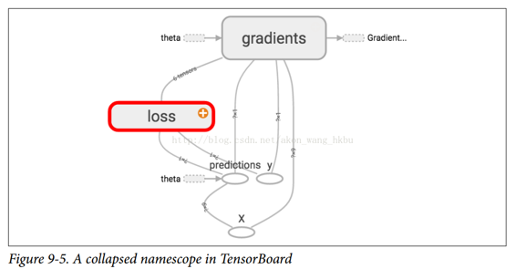例如，我們修改以前的代碼來定義名為`loss`的名稱作用域內的錯誤和`mse`操作： ```python with tf.name_scope("loss") as scope: error = y_pred - y mse = tf.reduce_mean(tf.square(error), name="mse") ``` 在作用域內定義的每個`op`的名稱現在以`loss/`為前綴： ```python >>> print(error.op.name) loss/sub >>> print(mse.op.name) loss/mse ``` 在 TensorBoard 中，`mse`和`error`節點現在出現在`loss`命名空間中，默認情況下會出現崩潰（圖 9-5）。 ![](https://img.kancloud.cn/57/ac/57acf62240ce85f7d5e262633c9a8422_566x295.png) 完整代碼 ```python import numpy as np from sklearn.datasets import fetch_california_housing import tensorflow as tf from sklearn.preprocessing import StandardScaler housing = fetch_california_housing() m, n = housing.data.shape print("數據集:{}行,{}列".format(m,n)) housing_data_plus_bias = np.c_[np.ones((m, 1)), housing.data] scaler = StandardScaler() scaled_housing_data = scaler.fit_transform(housing.data) scaled_housing_data_plus_bias = np.c_[np.ones((m, 1)), scaled_housing_data] from datetime import datetime now = datetime.utcnow().strftime("%Y%m%d%H%M%S") root_logdir = r"D://tf_logs" logdir = "{}/run-{}/".format(root_logdir, now) n_epochs = 1000 learning_rate = 0.01 X = tf.placeholder(tf.float32, shape=(None, n + 1), name="X") y = tf.placeholder(tf.float32, shape=(None, 1), name="y") theta = tf.Variable(tf.random_uniform([n + 1, 1], -1.0, 1.0, seed=42), name="theta") y_pred = tf.matmul(X, theta, name="predictions") def fetch_batch(epoch, batch_index, batch_size): np.random.seed(epoch * n_batches + batch_index) # not shown in the book indices = np.random.randint(m, size=batch_size) # not shown X_batch = scaled_housing_data_plus_bias[indices] # not shown y_batch = housing.target.reshape(-1, 1)[indices] # not shown return X_batch, y_batch with tf.name_scope("loss") as scope: error = y_pred - y mse = tf.reduce_mean(tf.square(error), name="mse") optimizer = tf.train.GradientDescentOptimizer(learning_rate=learning_rate) training_op = optimizer.minimize(mse) init = tf.global_variables_initializer() mse_summary = tf.summary.scalar('MSE', mse) file_writer = tf.summary.FileWriter(logdir, tf.get_default_graph()) n_epochs = 10 batch_size = 100 n_batches = int(np.ceil(m / batch_size)) with tf.Session() as sess: sess.run(init) for epoch in range(n_epochs): for batch_index in range(n_batches): X_batch, y_batch = fetch_batch(epoch, batch_index, batch_size) if batch_index % 10 == 0: summary_str = mse_summary.eval(feed_dict={X: X_batch, y: y_batch}) step = epoch * n_batches + batch_index file_writer.add_summary(summary_str, step) sess.run(training_op, feed_dict={X: X_batch, y: y_batch}) best_theta = theta.eval() file_writer.flush() file_writer.close() print("Best theta:") print(best_theta) ``` ![](https://img.kancloud.cn/24/19/24191caef4ab78a30a882ea46cc0904e_566x376.png) ## 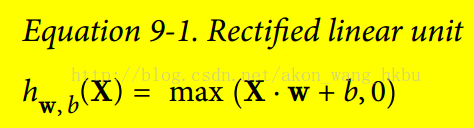模塊性假設您要創建一個圖，它的作用是將兩個整流線性單元（ReLU）的輸出值相加。 ReLU 計算一個輸入值的對應線性函數輸出值，如果為正，則輸出該結值，否則為 0，如等式 9-1 所示。 ![](https://img.kancloud.cn/fc/e5/fce51248e1c402bf1e3270e6d5ea8e47_474x128.png) 下面的代碼做這個工作，但是它是相當重復的： ```python n_features = 3 X = tf.placeholder(tf.float32, shape=(None, n_features), name="X") w1 = tf.Variable(tf.random_normal((n_features, 1)), name="weights1") w2 = tf.Variable(tf.random_normal((n_features, 1)), name="weights2") b1 = tf.Variable(0.0, name="bias1") b2 = tf.Variable(0.0, name="bias2") z1 = tf.add(tf.matmul(X, w1), b1, name="z1") z2 = tf.add(tf.matmul(X, w2), b2, name="z2") relu1 = tf.maximum(z1, 0., name="relu1") relu2 = tf.maximum(z1, 0., name="relu2") output = tf.add(relu1, relu2, name="output") ``` 這樣的重復代碼很難維護，容易出錯（實際上，這個代碼包含了一個剪貼錯誤，你發現了嗎？）如果你想添加更多的 ReLU，會變得更糟。幸運的是，TensorFlow 可以讓您保持 DRY（不要重復自己）：只需創建一個功能來構建 ReLU。以下代碼創建五個 ReLU 并輸出其總和（注意，`add_n()`創建一個計算張量列表之和的操作）： ```python def relu(X): w_shape = (int(X.get_shape()[1]), 1) w = tf.Variable(tf.random_normal(w_shape), name="weights") b = tf.Variable(0.0, name="bias") z = tf.add(tf.matmul(X, w), b, name="z") return tf.maximum(z, 0., name="relu") n_features = 3 X = tf.placeholder(tf.float32, shape=(None, n_features), name="X") relus = [relu(X) for i in range(5)] output = tf.add_n(relus, name="output") ``` 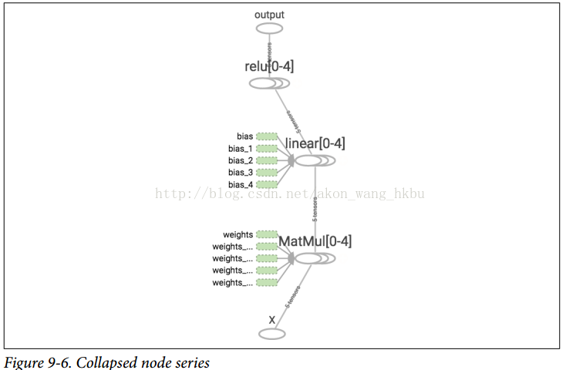請注意，創建節點時，TensorFlow 將檢查其名稱是否已存在，如果它已經存在，則會附加一個下劃線，后跟一個索引，以使該名稱是唯一的。因此，第一個 ReLU 包含名為`weights`，`bias`，`z`和`relu`的節點（加上其他默認名稱的更多節點，如`MatMul`）; 第二個 ReLU 包含名為`weights_1`，`bias_1`等節點的節點; 第三個 ReLU 包含名為 `weights_2`，`bias_2`的節點，依此類推。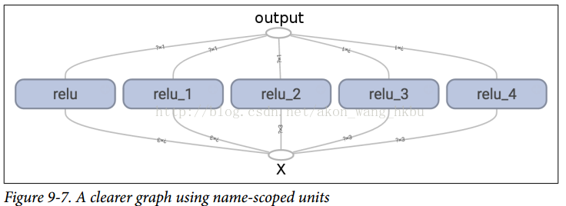 TensorBoard 識別這樣的系列并將它們折疊在一起以減少混亂（如圖 9-6 所示） ![](https://img.kancloud.cn/c2/ff/c2ffb199d40479252cf13b4688b4aec5_566x370.png) 使用名稱作用域，您可以使圖形更清晰。簡單地將`relu()`函數的所有內容移動到名稱作用域內。圖 9-7 顯示了結果圖。請注意，TensorFlow 還通過附加`_1`，`_2`等來提供名稱作用域的唯一名稱。 ```python def relu(X): with tf.name_scope("relu"): w_shape = (int(X.get_shape()[1]), 1) # not shown in the book w = tf.Variable(tf.random_normal(w_shape), name="weights") # not shown b = tf.Variable(0.0, name="bias") # not shown z = tf.add(tf.matmul(X, w), b, name="z") # not shown return tf.maximum(z, 0., name="max") # not shown ``` ![](https://img.kancloud.cn/58/b4/58b4f65f32f1bb0d844aab472804df33_566x206.png) ## 共享變量如果要在圖形的各個組件之間共享一個變量，一個簡單的選項是首先創建它，然后將其作為參數傳遞給需要它的函數。例如，假設要使用所有 ReLU 的共享閾值變量來控制 ReLU 閾值（當前硬編碼為 0）。您可以先創建該變量，然后將其傳遞給`relu()`函數： ```python reset_graph() def relu(X, threshold): with tf.name_scope("relu"): w_shape = (int(X.get_shape()[1]), 1) # not shown in the book w = tf.Variable(tf.random_normal(w_shape), name="weights") # not shown b = tf.Variable(0.0, name="bias") # not shown z = tf.add(tf.matmul(X, w), b, name="z") # not shown return tf.maximum(z, threshold, name="max") threshold = tf.Variable(0.0, name="threshold") X = tf.placeholder(tf.float32, shape=(None, n_features), name="X") relus = [relu(X, threshold) for i in range(5)] output = tf.add_n(relus, name="output") ``` 這很好:現在您可以使用閾值變量來控制所有 ReLU 的閾值。但是，如果有許多共享參數，比如這一項，那么必須一直將它們作為參數傳遞，這將是非常痛苦的。許多人創建了一個包含模型中所有變量的 Python 字典，并將其傳遞給每個函數。另一些則為每個模塊創建一個類（例如：一個使用類變量來處理共享參數的 ReLU 類）。另一種選擇是在第一次調用時將共享變量設置為`relu()`函數的屬性，如下所示: ```python def relu(X): with tf.name_scope("relu"): if not hasattr(relu, "threshold"): relu.threshold = tf.Variable(0.0, name="threshold") w_shape = int(X.get_shape()[1]), 1 # not shown in the book w = tf.Variable(tf.random_normal(w_shape), name="weights") # not shown b = tf.Variable(0.0, name="bias") # not shown z = tf.add(tf.matmul(X, w), b, name="z") # not shown return tf.maximum(z, relu.threshold, name="max") ``` TensorFlow 提供了另一個選項，這將提供比以前的解決方案稍微更清潔和更模塊化的代碼。首先要明白一點，這個解決方案很刁鉆難懂，但是由于它在 TensorFlow 中使用了很多，所以值得我們去深入細節。這個想法是使用`get_variable()`函數來創建共享變量，如果它還不存在，或者如果已經存在，則復用它。所需的行為（創建或復用）由當前`variable_scope()`的屬性控制。例如，以下代碼將創建一個名為`relu/threshold`的變量（作為標量，因為`shape = ()`，并使用 0.0 作為初始值）： ```python with tf.variable_scope("relu"): threshold = tf.get_variable("threshold", shape=(), initializer=tf.constant_initializer(0.0)) ``` 請注意，如果變量已經通過較早的`get_variable()`調用創建，則此代碼將引發異常。這種行為可以防止錯誤地復用變量。如果要復用變量，則需要通過將變量`scope`的復用屬性設置為`True`來明確說明（在這種情況下，您不必指定形狀或初始值）： ```python with tf.variable_scope("relu", reuse=True): threshold = tf.get_variable("threshold") ``` 該代碼將獲取現有的`relu/threshold`變量，如果不存在會引發異常（如果沒有使用`get_variable()`創建）。或者，您可以通過調用`scope`的`reuse_variables()`方法將復用屬性設置為`true`： ```python with tf.variable_scope("relu") as scope: scope.reuse_variables() threshold = tf.get_variable("threshold") ``` 一旦重新使用設置為`True`，它將不能在塊內設置為`False`。而且，如果在其中定義其他變量作用域，它們將自動繼承`reuse = True`。最后，只有通過`get_variable()`創建的變量才可以這樣復用. 現在，您擁有所有需要的部分，使`relu()`函數訪問閾值變量，而不必將其作為參數傳遞： ```python def relu(X): with tf.variable_scope("relu", reuse=True): threshold = tf.get_variable("threshold") w_shape = int(X.get_shape()[1]), 1 # not shown w = tf.Variable(tf.random_normal(w_shape), name="weights") # not shown b = tf.Variable(0.0, name="bias") # not shown z = tf.add(tf.matmul(X, w), b, name="z") # not shown return tf.maximum(z, threshold, name="max") X = tf.placeholder(tf.float32, shape=(None, n_features), name="X") with tf.variable_scope("relu"): threshold = tf.get_variable("threshold", shape=(), initializer=tf.constant_initializer(0.0)) relus = [relu(X) for relu_index in range(5)] output = tf.add_n(relus, name="output") ``` 該代碼首先定義`relu()`函數，然后創建`relu/threshold`變量（作為標量，稍后將被初始化為 0.0），并通過調用`relu()`函數構建五個ReLU。`relu()`函數復用`relu/threshold`變量，并創建其他 ReLU 節點。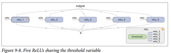使用`get_variable()`創建的變量始終以其`variable_scope`的名稱作為前綴命名（例如，`relu/threshold`），但對于所有其他節點（包括使用`tf.Variable()`創建的變量），變量作用域的行為就像一個新名稱的作用域。特別是，如果已經創建了具有相同名稱的名稱作用域，則添加后綴以使該名稱是唯一的。例如，在前面的代碼中創建的所有節點（閾值變量除外）的名稱前綴為`relu_1/`到`relu_5/`，如圖 9-8 所示。 ![](https://img.kancloud.cn/44/9f/449fa5abb0c64b24412f616bd9ccd964_566x175.png) 不幸的是，必須在`relu()`函數之外定義閾值變量，其中 ReLU 代碼的其余部分都駐留在其中。要解決此問題，以下代碼在第一次調用時在`relu()`函數中創建閾值變量，然后在后續調用中重新使用。現在，`relu()`函數不必擔心名稱作用域或變量共享：它只是調用`get_variable()`，它將創建或復用閾值變量（它不需要知道是哪種情況）。其余的代碼調用`relu()`五次，確保在第一次調用時設置`reuse = False`，而對于其他調用來說，`reuse = True`。 ```python def relu(X): threshold = tf.get_variable("threshold", shape=(), initializer=tf.constant_initializer(0.0)) w_shape = (int(X.get_shape()[1]), 1) # not shown in the book w = tf.Variable(tf.random_normal(w_shape), name="weights") # not shown b = tf.Variable(0.0, name="bias") # not shown z = tf.add(tf.matmul(X, w), b, name="z") # not shown return tf.maximum(z, threshold, name="max") X = tf.placeholder(tf.float32, shape=(None, n_features), name="X") relus = [] for relu_index in range(5): with tf.variable_scope("relu", reuse=(relu_index >= 1)) as scope: relus.append(relu(X)) output = tf.add_n(relus, name="output") ``` 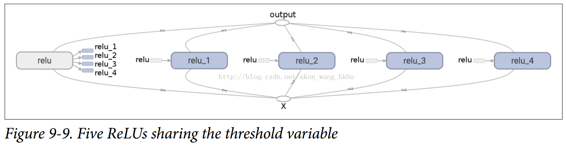生成的圖形與之前略有不同，因為共享變量存在于第一個 ReLU 中（見圖 9-9）。 ![](https://img.kancloud.cn/67/e9/67e90655badc9bb95d215b8c6ac137e0_566x145.png) TensorFlow 的這個介紹到此結束。我們將在以下章節中討論更多高級課題，特別是與深層神經網絡，卷積神經網絡和遞歸神經網絡相關的許多操作，以及如何使用多線程，隊列，多個 GPU 以及如何將 TensorFlow 擴展到多臺服務器。