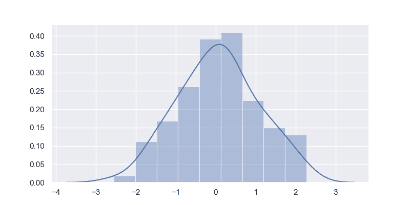
# Seaborn 分布圖 > 原文： [https://pythonbasics.org/seaborn-distplot/](https://pythonbasics.org/seaborn-distplot/) 通過 Seaborn 分布圖，您可以顯示帶有線條的直方圖。 這可以以各種變化形式顯示。 我們將 Seaborn 與 Python 繪圖模塊 Matplotlib 結合使用。 分布圖繪制觀測值的單變量分布。 `distplot()`函數將 Matplotlib `hist`函數與 Seaborn `kdeplot()`和`rugplot()`函數結合在一起。 ## 示例 ### 分布圖示例 下圖顯示了一個簡單的分布。 它使用`random.randn()`創建隨機值。如果您也手動定義值，它將起作用。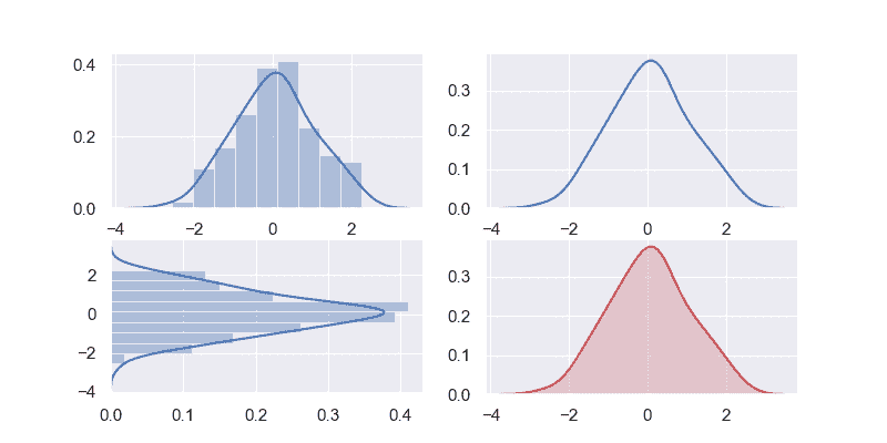 ```py import matplotlib.pyplot as plt import seaborn as sns, numpy as np sns.set(rc={"figure.figsize": (8, 4)}); np.random.seed(0) x = np.random.randn(100) ax = sns.distplot(x) plt.show() ```  ### 分布圖示例 您可以顯示分布圖的各種變化。 我們使用`pylab`模塊中的`subplot()`方法來一次顯示 4 種變化。 通過更改`distplot()`方法中的參數，您可以創建完全不同的視圖。 您可以使用這些參數來更改顏色，方向等。 ```py import matplotlib.pyplot as plt import seaborn as sns, numpy as np from pylab import * sns.set(rc={"figure.figsize": (8, 4)}); np.random.seed(0) x = np.random.randn(100) subplot(2,2,1) ax = sns.distplot(x) subplot(2,2,2) ax = sns.distplot(x, rug=False, hist=False) subplot(2,2,3) ax = sns.distplot(x, vertical=True) subplot(2,2,4) ax = sns.kdeplot(x, shade=True, color="r") plt.show() ```  [下載示例](https://gum.co/mpdp) ### Seaborn 分布 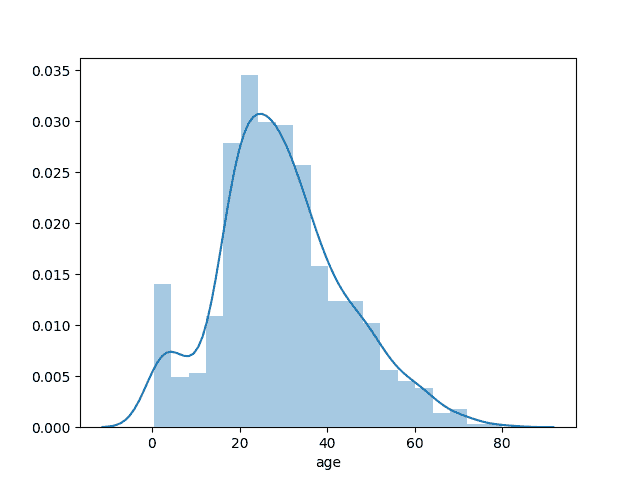您也可以在直方圖中顯示 Seaborn 的標準數據集。這是一個很大的數據集，因此僅占用一列。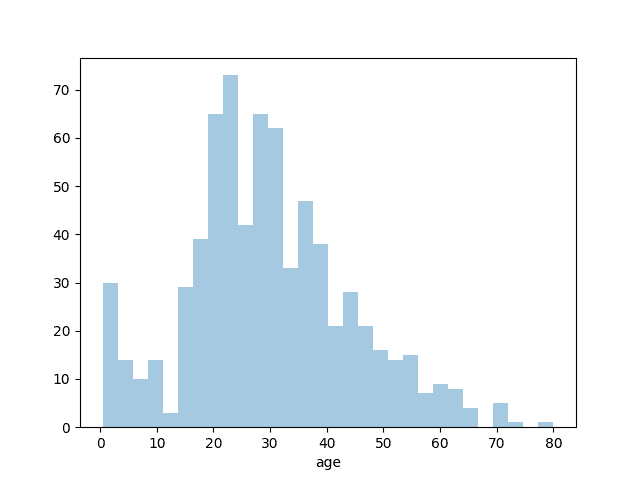 ```py import matplotlib.pyplot as plt import seaborn as sns titanic=sns.load_dataset('titanic') age1=titanic['age'].dropna() sns.distplot(age1) plt.show() ```  ### 分布圖容器 如果您想更改桶的數量或隱藏行，也可以。當調用方法`distplot()`時，您可以傳遞箱數并告訴直線（kde）不可見。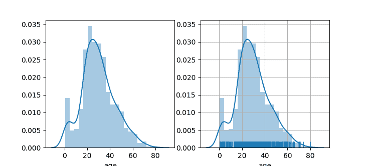 ```py import matplotlib.pyplot as plt import seaborn as sns titanic=sns.load_dataset('titanic') age1=titanic['age'].dropna() sns.distplot(age1,bins=30,kde=False) plt.show() ```  ### Seaborn 不同的繪圖 下面的示例顯示了其他一些分布圖示例。 您通過`grid(True)`方法調用激活了一個網格。 ```py import matplotlib.pyplot as plt import seaborn as sns titanic=sns.load_dataset('titanic') age1=titanic['age'].dropna() fig,axes=plt.subplots(1,2) sns.distplot(age1,ax=axes[0]) plt.grid(True) sns.distplot(age1,rug=True,ax=axes[1]) plt.show() ```  [下載示例](https://gum.co/mpdp)