# seaborn.jointplot > 譯者：[Stuming](https://github.com/Stuming) ```py seaborn.jointplot(x, y, data=None, kind='scatter', stat_func=None, color=None, height=6, ratio=5, space=0.2, dropna=True, xlim=None, ylim=None, joint_kws=None, marginal_kws=None, annot_kws=None, **kwargs) ``` 繪制兩個變量的雙變量及單變量圖。 這個函數提供調用[`JointGrid`](seaborn.JointGrid.html#seaborn.JointGrid "seaborn.JointGrid")類的便捷接口，以及一些封裝好的繪圖類型。這是一個輕量級的封裝，如果需要更多的靈活性，應當直接使用[`JointGrid`](seaborn.JointGrid.html#seaborn.JointGrid "seaborn.JointGrid"). 參數：`x, y`：strings 或者 vectors > `data`中的數據或者變量名。 `data`：DataFrame, 可選 > 當`x`和`y`為變量名時的 DataFrame. `kind`：{ “scatter” | “reg” | “resid” | “kde” | “hex” }, 可選 > 繪制圖像的類型。 `stat_func`：可調用的，或者 None, 可選 > 已過時 `color`：matplotlib 顏色, 可選 > 用于繪制元素的顏色。 `height`：numeric, 可選 > 圖像的尺寸（方形）。 `ratio`：numeric, 可選 > 中心軸的高度與側邊軸高度的比例 `space`：numeric, 可選 > 中心和側邊軸的間隔大小 `dropna`：bool, 可選 > 如果為 True, 移除`x`和`y`中的缺失值。 `{x, y}lim`：two-tuples, 可選 > 繪制前設置軸的范圍。 `{joint, marginal, annot}_kws`：dicts, 可選 > 額外的關鍵字參數。 `kwargs`：鍵值對 > 額外的關鍵字參數會被傳給繪制中心軸圖像的函數，取代`joint_kws`字典中的項。 返回值：`grid`：[`JointGrid`](seaborn.JointGrid.html#seaborn.JointGrid "seaborn.JointGrid") > [`JointGrid`](seaborn.JointGrid.html#seaborn.JointGrid "seaborn.JointGrid")對象. 參考 繪制圖像的 Grid 類。如果需要更多的靈活性，可以直接使用 Grid 類。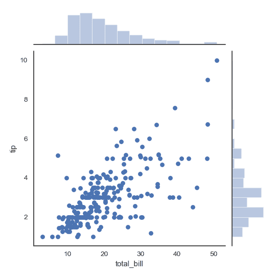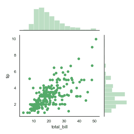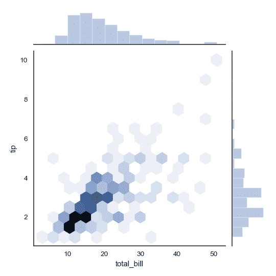 示例 繪制帶有側邊直方圖的散點圖: ```py >>> import numpy as np, pandas as pd; np.random.seed(0) >>> import seaborn as sns; sns.set(style="white", color_codes=True) >>> tips = sns.load_dataset("tips") >>> g = sns.jointplot(x="total_bill", y="tip", data=tips) ```  添加回歸線及核密度擬合: ```py >>> g = sns.jointplot("total_bill", "tip", data=tips, kind="reg") ```  將散點圖替換為六角形箱體圖: ```py >>> g = sns.jointplot("total_bill", "tip", data=tips, kind="hex") ```  將散點圖和直方圖替換為密度估計，并且將側邊軸與中心軸對齊: ```py >>> iris = sns.load_dataset("iris") >>> g = sns.jointplot("sepal_width", "petal_length", data=iris, ... 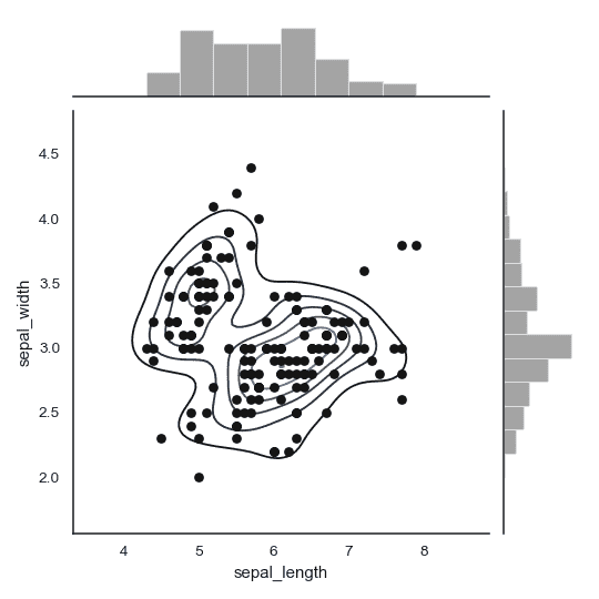kind="kde", space=0, color="g") ```  繪制散點圖，添加中心密度估計: ```py >>> g = (sns.jointplot("sepal_length", "sepal_width", ... data=iris, color="k") ... 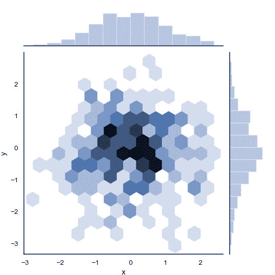.plot_joint(sns.kdeplot, zorder=0, n_levels=6)) ```  不適用 Pandas, 直接傳輸向量，隨后給軸命名: ```py >>> x, y = np.random.randn(2, 300) >>> g = (sns.jointplot(x, y, kind="hex") ... .set_axis_labels("x", "y")) ```  繪制側邊圖空間更大的圖像: ```py >>> g = sns.jointplot("total_bill", "tip", data=tips, ... 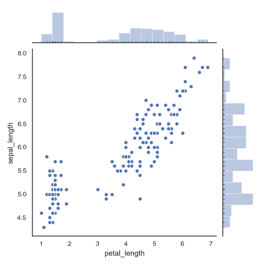height=5, ratio=3, color="g") ```  傳遞關鍵字參數給后續繪制函數: ```py >>> g = sns.jointplot("petal_length", "sepal_length", data=iris, ... marginal_kws=dict(bins=15, rug=True), ... annot_kws=dict(stat="r"), ... s=40, edgecolor="w", linewidth=1) ```