# 使用程序最小化損失 > 原文：[https://www.bookbookmark.ds100.org/ch/11/gradient_basics.html](https://www.bookbookmark.ds100.org/ch/11/gradient_basics.html) ``` # HIDDEN # Clear previously defined variables %reset -f # Set directory for data loading to work properly import os os.chdir(os.path.expanduser('~/notebooks/11')) ``` ``` # HIDDEN import warnings # Ignore numpy dtype warnings. These warnings are caused by an interaction # between numpy and Cython and can be safely ignored. # Reference: https://stackoverflow.com/a/40846742 warnings.filterwarnings("ignore", message="numpy.dtype size changed") warnings.filterwarnings("ignore", message="numpy.ufunc size changed") import numpy as np import matplotlib.pyplot as plt import pandas as pd import seaborn as sns %matplotlib inline import ipywidgets as widgets from ipywidgets import interact, interactive, fixed, interact_manual import nbinteract as nbi sns.set() sns.set_context('talk') np.set_printoptions(threshold=20, precision=2, suppress=True) pd.options.display.max_rows = 7 pd.options.display.max_columns = 8 pd.set_option('precision', 2) # This option stops scientific notation for pandas # pd.set_option('display.float_format', '{:.2f}'.format) ``` ``` # HIDDEN def mse(theta, y_vals): return np.mean((y_vals - theta) ** 2) def points_and_loss(y_vals, xlim, loss_fn): thetas = np.arange(xlim[0], xlim[1] + 0.01, 0.05) losses = [loss_fn(theta, y_vals) for theta in thetas] plt.figure(figsize=(9, 2)) ax = plt.subplot(121) sns.rugplot(y_vals, height=0.3, ax=ax) plt.xlim(*xlim) plt.title('Points') plt.xlabel('Tip Percent') ax = plt.subplot(122) plt.plot(thetas, losses) plt.xlim(*xlim) plt.title(loss_fn.__name__) plt.xlabel(r'$ \theta $') plt.ylabel('Loss') plt.legend() ``` 讓我們回到常量模型： $$ \theta = C $$ 我們將使用均方誤差損失函數： $$ \begin{aligned} L(\theta, \textbf{y}) &= \frac{1}{n} \sum_{i = 1}^{n}(y_i - \theta)^2\\ \end{aligned} $$ 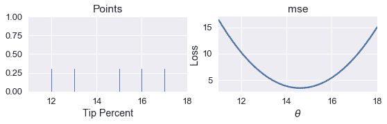為了簡單起見，我們將使用數據集$\textbf y=[12，13，15，16，17]$。從上一章的分析方法中我們知道，MSE 的最小$\theta$是$\text mean（\textbf y）=14.6$。讓我們看看是否可以通過編寫程序找到相同的值。 如果我們寫得好，我們將能夠在任何損失函數上使用相同的程序，以便找到$\theta$的最小值，包括數學上復雜的 Huber 損失： $$ L_\alpha(\theta, \textbf{y}) = \frac{1}{n} \sum_{i=1}^n \begin{cases} \frac{1}{2}(y_i - \theta)^2 & | y_i - \theta | \le \alpha \\ \alpha ( |y_i - \theta| - \frac{1}{2}\alpha ) & \text{otherwise} \end{cases} $$ 首先，我們創建數據點的地毯圖。在地毯圖的右側，我們繪制了不同值（$\theta$）的 MSE。 ``` # HIDDEN pts = np.array([12, 13, 15, 16, 17]) points_and_loss(pts, (11, 18), mse) ```  我們如何編寫一個程序來自動找到$\theta$的最小值？最簡單的方法是計算許多值的損失。然后，我們可以返回導致最小損失的\theta$值。 我們定義了一個名為`simple_minimize`的函數，它接受一個丟失函數、一個數據點數組和一個要嘗試的$\theta$值數組。 ``` def simple_minimize(loss_fn, dataset, thetas): ''' Returns the value of theta in thetas that produces the least loss on a given dataset. ''' losses = [loss_fn(theta, dataset) for theta in thetas] return thetas[np.argmin(losses)] ``` 然后，我們可以定義一個函數來計算 mse 并將其傳遞到`simple_minimize`。 ``` def mse(theta, dataset): return np.mean((dataset - theta) ** 2) dataset = np.array([12, 13, 15, 16, 17]) thetas = np.arange(12, 18, 0.1) simple_minimize(mse, dataset, thetas) ``` ``` 14.599999999999991 ``` 這接近預期值： ``` # Compute the minimizing theta using the analytical formula np.mean(dataset) ``` ``` 14.6 ``` 現在，我們可以定義一個函數來計算 Huber 損失，并將損失與$\theta$進行比較。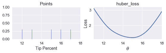 ``` def huber_loss(theta, dataset, alpha = 1): d = np.abs(theta - dataset) return np.mean( np.where(d < alpha, (theta - dataset)**2 / 2.0, alpha * (d - alpha / 2.0)) ) ``` ``` # HIDDEN points_and_loss(pts, (11, 18), huber_loss) ```  雖然我們可以看到，$\theta$的最小值應該接近 15，但是我們沒有直接為 Huber 損失找到$\theta$的分析方法。相反，我們可以使用`simple_minimize`函數。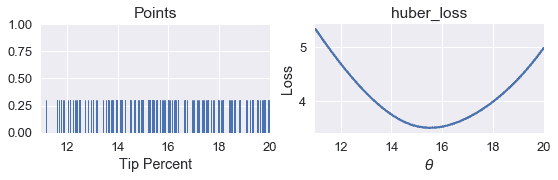 ``` simple_minimize(huber_loss, dataset, thetas) ``` ``` 14.999999999999989 ``` 現在，我們可以返回到 Tip 百分比的原始數據集，并使用 Huber 損失找到$\theta$的最佳值。 ``` tips = sns.load_dataset('tips') tips['pcttip'] = tips['tip'] / tips['total_bill'] * 100 tips.head() ``` | | 賬單合計 | 提示 | 性別 | 吸煙者 | 白天 | 時間 | 大小 | PCTIP | | --- | --- | --- | --- | --- | --- | --- | --- | --- | | 零 | 十六點九九 | 1.01 年 | 女性 | 不 | 太陽 | 晚餐 | 二 | 5.944673 頁 | | --- | --- | --- | --- | --- | --- | --- | --- | --- | | 1 個 | 十點三四 | 一點六六 | 男性 | No | Sun | Dinner | 三 | 16.054159 頁 | | --- | --- | --- | --- | --- | --- | --- | --- | --- | | 二 | 二十一點零一 | 3.50 美元 | Male | No | Sun | Dinner | 3 | 16.658734 | | --- | --- | --- | --- | --- | --- | --- | --- | --- | | 三 | 二十三點六八 | 三點三一 | Male | No | Sun | Dinner | 2 | 13.978041 | | --- | --- | --- | --- | --- | --- | --- | --- | --- | | 四 | 二十四點五九 | 三點六一 | Female | No | Sun | Dinner | 四 | 14.680765 個 | | --- | --- | --- | --- | --- | --- | --- | --- | --- | ``` # HIDDEN points_and_loss(tips['pcttip'], (11, 20), huber_loss) ```  ``` simple_minimize(huber_loss, tips['pcttip'], thetas) ``` ``` 15.499999999999988 ``` 我們可以看到，使用 Huber 損失給我們帶來了\theta=15.5 美元。現在，我們可以比較 mse、mae 和 huber 損失的最小$\hat \theta 值。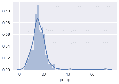 ``` print(f" MSE: theta_hat = {tips['pcttip'].mean():.2f}") print(f" MAE: theta_hat = {tips['pcttip'].median():.2f}") print(f" Huber loss: theta_hat = 15.50") ``` ``` MSE: theta_hat = 16.08 MAE: theta_hat = 15.48 Huber loss: theta_hat = 15.50 ``` 我們可以看到，Huber 損失更接近 MAE，因為它受 Tip 百分比分布右側的異常值影響較小： ``` sns.distplot(tips['pcttip'], bins=50); ```  ## 與`simple_minimize`[?](#Issues-with-simple_minimize)有關的問題 雖然`simple_minimize`允許我們最小化損失函數，但它有一些缺陷，使其不適合一般用途。它的主要問題是，它只使用預先確定的$theta$值進行測試。例如，在我們上面使用的代碼片段中，我們必須在 12 到 18 之間手動定義$\theta$值。 ``` dataset = np.array([12, 13, 15, 16, 17]) thetas = np.arange(12, 18, 0.1) simple_minimize(mse, dataset, thetas) ``` 我們如何知道檢查 12 到 18 之間的范圍？我們必須手動檢查損耗函數的曲線圖，并看到在這個范圍內有一個最小值。當我們為模型增加額外的復雜性時，這個過程變得不切實際。此外，我們在上面的代碼中手動指定了 0.1 的步長。然而，如果$\theta$的最佳值是 12.043，我們的`simple_minimize`函數將四舍五入到 12.00，即 0.1 的最接近倍數。 我們可以使用一個名為 _ 梯度下降 _ 的方法同時解決這兩個問題。