# 評估 Logistic 模型 > 原文：[https://www.bookbookmark.ds100.org/ch/17/classification_sensitivity_specificity.html](https://www.bookbookmark.ds100.org/ch/17/classification_sensitivity_specificity.html) ``` # HIDDEN # Clear previously defined variables %reset -f # Set directory for data loading to work properly import os os.chdir(os.path.expanduser('~/notebooks/17')) ``` ``` # HIDDEN import warnings # Ignore numpy dtype warnings. These warnings are caused by an interaction # between numpy and Cython and can be safely ignored. # Reference: https://stackoverflow.com/a/40846742 warnings.filterwarnings("ignore", message="numpy.dtype size changed") warnings.filterwarnings("ignore", message="numpy.ufunc size changed") import numpy as np import matplotlib.pyplot as plt import pandas as pd import seaborn as sns %matplotlib inline import ipywidgets as widgets from ipywidgets import interact, interactive, fixed, interact_manual import nbinteract as nbi sns.set() sns.set_context('talk') np.set_printoptions(threshold=20, precision=2, suppress=True) pd.options.display.max_rows = 7 pd.options.display.max_columns = 8 pd.set_option('precision', 2) # This option stops scientific notation for pandas # pd.set_option('display.float_format', '{:.2f}'.format) ``` ``` # HIDDEN from sklearn.feature_extraction import DictVectorizer from sklearn.model_selection import train_test_split from sklearn.linear_model import LogisticRegression from sklearn.metrics import confusion_matrix emails=pd.read_csv('selected_emails.csv', index_col=0) ``` ``` # HIDDEN def words_in_texts(words, texts): ''' Args: words (list-like): words to find texts (Series): strings to search in Returns: NumPy array of 0s and 1s with shape (n, p) where n is the number of texts and p is the number of words. ''' indicator_array = np.array([texts.str.contains(word) * 1 for word in words]).T # YOUR CODE HERE return indicator_array ``` 雖然我們在前面的章節中使用分類準確度來評估我們的 Logistic 模型，但是僅使用準確度就有一些嚴重的缺陷，我們在這一章節中對此進行了探討。為了解決這些問題，我們引入了一個更有用的度量來評估分類器性能：曲線下面積（AUC）度量。 假設我們有一個 1000 封郵件的數據集，它們被標記為垃圾郵件或火腿（不是垃圾郵件），我們的目標是建立一個分類器，將未來的垃圾郵件與火腿電子郵件區分開來。數據包含在下面顯示的`emails`數據框中： ``` emails ``` | | 身體 | 垃圾郵件 | | --- | --- | --- | | 零 | \嗨，伙計們，我一直在嘗試設置 bu… | 零 | | --- | --- | --- | | 1 個 | 哈哈。我想她不想讓每個人都知道… | 0 | | --- | --- | --- | | 二 | 這篇來自 nytimes.com 的文章已發送… | 0 | | --- | --- | --- | | …… | …… | ... | | --- | --- | --- | | 997 年 | &lt；html&gt；\n&lt；head&gt；\n&lt；meta http equiv=“conten…” | 1 個 | | --- | --- | --- | | 九百九十八 | &lt；html&gt；\n&lt；head&gt；\n&lt；/head&gt；\n&lt；body&gt；\n\n&lt；cente… | 1 | | --- | --- | --- | | 999 個 | \ n&lt；html&gt；\n\n&lt；head&gt；\n&lt；meta http equiv=3d“合作… | 1 | | --- | --- | --- | 1000 行×2 列 每一行包含`body`列中的電子郵件正文和`spam`列中的垃圾郵件指示器，如果電子郵件是 ham，則為`0`，如果是垃圾郵件，則為`1`。 讓我們比較三種不同分類器的性能： * `ham_only`：將每個電子郵件標記為 ham。 * `spam_only`：將每封電子郵件標記為垃圾郵件。 * `words_list_model`：根據電子郵件正文中的某些詞預測“ham”或“spam”。 假設我們有一個單詞列表`words_list`我們認為在垃圾郵件中很常見：“請”、“點擊”、“錢”、“生意”和“刪除”。我們使用以下過程構造`words_list_model`：如果`words_list`中的$i$th 字包含在電子郵件正文中，則通過將向量的$i$th 項設置為 1，否則設置為 0，將每個電子郵件轉換為特征向量。例如，使用我們選擇的五個字和電子郵件正文“請通過 Tomo 刪除”。rrow“，特征向量將為$[1，0，0，0，1]$。此過程生成`1000 X 5`功能矩陣$\textbf x$。 下面的代碼塊顯示分類器的精度。為了簡潔起見，省略了模型創建和培訓。 ``` # HIDDEN words_list = ['please', 'click', 'money', 'business', 'remove'] X = pd.DataFrame(words_in_texts(words_list, emails['body'].str.lower())).as_matrix() y = emails['spam'].as_matrix() # Train-test split X_train, X_test, y_train, y_test = train_test_split( X, y, random_state=41, test_size=0.2 ) #Fit the model words_list_model = LogisticRegression(fit_intercept=True) words_list_model.fit(X_train, y_train) y_prediction_words_list = words_list_model.predict(X_test) y_prediction_ham_only = np.zeros(len(y_test)) y_prediction_spam_only = np.ones(len(y_test)) ``` ``` from sklearn.metrics import accuracy_score # Our selected words words_list = ['please', 'click', 'money', 'business'] print(f'ham_only test set accuracy: {np.round(accuracy_score(y_prediction_ham_only, y_test), 3)}') print(f'spam_only test set accuracy: {np.round(accuracy_score(y_prediction_spam_only, y_test), 3)}') print(f'words_list_model test set accuracy: {np.round(accuracy_score(y_prediction_words_list, y_test), 3)}') ``` ``` ham_only test set accuracy: 0.96 spam_only test set accuracy: 0.04 words_list_model test set accuracy: 0.96 ``` 使用`words_list_model`可以正確分類 96%的測試集電子郵件。雖然這一精確度似乎很高，但通過簡單地將所有東西標記為火腿，HTG1 達到了同樣的精確度。這是值得關注的原因，因為數據表明我們完全可以在沒有垃圾郵件過濾器的情況下做得同樣好。 正如上述精度所示，僅模型精度就可能是模型性能的誤導性指標。我們可以使用**混淆矩陣**更深入地理解模型的預測。二元分類器的混淆矩陣是一個二乘二的 heatmap，它包含一個軸上的模型預測和另一個軸上的實際標簽。 混淆矩陣中的每個條目表示分類器的可能結果。如果將垃圾郵件輸入到分類器，則有兩種可能的結果： * **真陽性**（左上角的條目）：模型用陽性類（spam）正確地標記了它。 * **false negative**（右上角的條目）：模型將其錯誤地標記為負類（ham），但它確實屬于正類（spam）。在我們的例子中，一個錯誤的否定意味著一封垃圾郵件被錯誤地標記為火腿，并最終進入收件箱。 同樣，如果一封火腿電子郵件被輸入到分類器，有兩種可能的結果。 * **假陽性**（左下角的條目）：模型用陽性類（spam）誤導了它，但它確實屬于陰性類（ham）。在我們的例子中，假陽性意味著一封火腿電子郵件會被標記為垃圾郵件并從收件箱中過濾掉。 * **真負**（右下角輸入）：模型正確地用負類（ham）標記它。 假陽性和假陰性的成本取決于情況。對于電子郵件分類，誤報會導致重要的電子郵件被過濾掉，因此它們比誤報更糟糕，因為垃圾郵件會在收件箱中結束。然而，在醫療環境中，診斷測試中的假陰性比假陽性更為重要。 我們將使用 Scikit Learn 的[混淆矩陣函數](http://scikit-learn.org/stable/modules/generated/sklearn.metrics.confusion_matrix.html#sklearn.metrics.confusion_matrix)為訓練數據集上的三個模型構造混淆矩陣。`ham_only`混淆矩陣如下： ``` # HIDDEN def plot_confusion_matrix(cm, classes, normalize=False, title='Confusion matrix', cmap=plt.cm.Blues): """ This function prints and plots the confusion matrix. Normalization can be applied by setting `normalize=True`. """ import itertools if normalize: cm = cm.astype('float') / cm.sum(axis=1)[:, np.newaxis] # print("Normalized confusion matrix") # else: # print('Confusion matrix, without normalization') # print(cm) plt.imshow(cm, interpolation='nearest', cmap=cmap) plt.title(title) plt.colorbar() tick_marks = np.arange(len(classes)) plt.xticks(tick_marks, classes, rotation=45) plt.yticks(tick_marks, classes) fmt = '.2f' if normalize else 'd' thresh = cm.max() / 2. for i, j in itertools.product(range(cm.shape[0]), range(cm.shape[1])): plt.text(j, i, format(cm[i, j], fmt), horizontalalignment="center", color="white" if cm[i, j] > thresh else "black") plt.tight_layout() plt.ylabel('True label') plt.xlabel('Predicted label') plt.grid(False) ham_only_y_pred = np.zeros(len(y_train)) spam_only_y_pred = np.ones(len(y_train)) words_list_model_y_pred = words_list_model.predict(X_train) ``` ``` from sklearn.metrics import confusion_matrix class_names = ['Spam', 'Ham'] ham_only_cnf_matrix = confusion_matrix(y_train, ham_only_y_pred, labels=[1, 0]) plot_confusion_matrix(ham_only_cnf_matrix, classes=class_names, title='ham_only Confusion Matrix') ```  將一行中的數量相加表示培訓數據集中有多少電子郵件屬于相應的類： * 真標簽=垃圾郵件（第一行）：真陽性（0）和假陰性（42）的總和顯示培訓數據集中有 42 封垃圾郵件。 * 真標簽=ham（第二行）：假陽性（0）和真陰性（758）的總和顯示訓練數據集中有 758 封 ham 電子郵件。 對列中的數量求和表示分類器在相應類中預測的電子郵件數： * 預測標簽=垃圾郵件（第一列）：真陽性（0）和假陽性（0）的總和顯示`ham_only`預測培訓數據集中有 0 封垃圾郵件。 * 預測標簽=ham（第二列）：假陰性（42）和真陰性（758）的總和顯示`ham_only`預測培訓數據集中有 800 封 ham 電子郵件。 我們可以看到`ham_only`的高精度為$左（\frac 758 800 \約 95 右）$因為在總共 800 封電子郵件中，培訓數據集中有 758 封 HAM 電子郵件。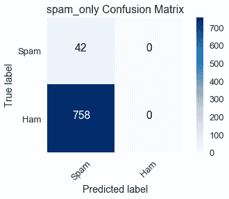 ``` spam_only_cnf_matrix = confusion_matrix(y_train, spam_only_y_pred, labels=[1, 0]) plot_confusion_matrix(spam_only_cnf_matrix, classes=class_names, title='spam_only Confusion Matrix') ```  另一個極端是，`spam_only`預測訓練數據集沒有 ham 電子郵件，混淆矩陣顯示這與 758 個誤報的事實相差甚遠。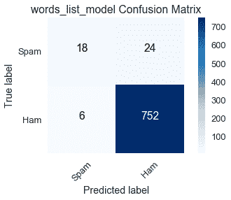 我們的主要興趣是`words_list_model`的混淆矩陣： ``` words_list_model_cnf_matrix = confusion_matrix(y_train, words_list_model_y_pred, labels=[1, 0]) plot_confusion_matrix(words_list_model_cnf_matrix, classes=class_names, title='words_list_model Confusion Matrix') ```  行總數與預期的`ham_only`和`spam_only`混淆矩陣相匹配，因為訓練數據集中的真實標簽對所有模型都是不變的。 在 42 封垃圾郵件中，`words_list_model`正確地分類了 18 封，這是一個糟糕的性能。它的高精度受到大量真實否定的支持，但這是不夠的，因為它不符合可靠過濾垃圾郵件的目的。 此電子郵件數據集是**類不平衡數據集**的一個示例，其中絕大多數標簽屬于一個類而不是另一個類。在這種情況下，我們的大多數電子郵件都是火腿。另一個常見的階級失衡的例子是，當一個群體的疾病發生頻率較低時，疾病檢測。一項醫學測試總是得出這樣的結論：病人沒有這種疾病會有很高的準確性，因為大多數病人確實沒有這種疾病，但是它無法識別出患有這種疾病的人，這就使得它毫無用處。 我們現在轉向敏感性和特異性，這兩個指標更適合評估類不平衡數據集。 ### 靈敏度[?](#Sensitivity) **靈敏度**（也稱為**真陽性率**）測量屬于分類器正確標記的陽性類的數據比例。 $$ \text{Sensitivity} = \frac{TP}{TP + FN} $$ 從我們對混淆矩陣的討論中，您應該將表達式$tp+fn$識別為第一行中條目的總和，它等于數據集中屬于正類的實際數據點數量。使用混淆矩陣可以很容易地比較模型的敏感性： * `ham_only`：$\frac 0 0+42=0$ * `spam_only`：$\frac 42 42+0=1$ * `words_list_model`：$\frac 18 18+24 \約 429$ 因為`ham_only`沒有真陽性，所以它的靈敏度值可能是 0。另一方面，`spam_only`的準確度非常低，但它的靈敏度值可能是 1，因為它正確地標記了所有垃圾郵件。`words_list_model`的低敏感度表明它經常無法標記垃圾郵件；然而，它的表現明顯優于`ham_only`。 ### 特異性 **特異性**（也稱為**真負率**）測量屬于分類器正確標記的負類的數據比例。 $$ \text{Specificity} = \frac{TN}{TN + FP} $$ 表達式$tn+fp$等于數據集中屬于負類的實際數據點數。同樣，混淆矩陣有助于比較模型的特性： * `ham_only`：$\frac 758 758+0=1$ * `spam_only`：$\frac 0 0+758=0$ * `words_list_model`：$\frac 752 752+6 \約 992$ 與敏感性一樣，最差和最好的特異性分別為 0 和 1。注意，`ham_only`有最好的特異性和最差的敏感性，而`spam_only`有最差的特異性和最好的敏感性。由于這些模型只預測一個標簽，它們將錯誤分類另一個標簽的所有實例，這反映在極端的敏感性和特異性值中。對于`words_list_model`來說，差距要小得多。 雖然敏感性和特異性似乎描述了分類器的不同特征，但我們使用分類閾值在這兩個指標之間建立了重要的聯系。 ### 分類閾值[?](#Classification-Threshold) **分類閾值**是一個值，用于確定將數據點分配給什么類；位于閾值兩側的點用不同的類進行標記。回想一下，邏輯回歸輸出數據點屬于正類的概率。如果此概率大于閾值，則數據點標記為正類，如果低于閾值，則數據點標記為負類。對于我們的例子，讓$F_ \那\ theta 作為邏輯模型，讓$C$作為閾值。如果$F_ \Theta（x）&gt；C$標記，$X$標記為垃圾郵件；如果$F \Theta（x）&lt；C$標記，$X$標記為火腿。SciKit Learn 通過默認為負類打破了聯系，因此如果$f \that \theta（x）=c$，$x$標記為 ham。 我們可以通過創建一個混淆矩陣，用分類閾值$C$來評估模型的性能。本節前面顯示的`words_list_model`混淆矩陣使用 SciKit 學習的默認閾值$C=0.50$。 將閾值提高到$C=0.70 美元，這意味著如果概率$F \that \theta（x）$大于.70，我們會將電子郵件$X$標記為垃圾郵件，從而導致以下混淆矩陣： ``` # HIDDEN words_list_prediction_probabilities = words_list_model.predict_proba(X_train)[:, 1] words_list_predictions = [1 if pred >= .70 else 0 for pred in words_list_prediction_probabilities] high_classification_threshold = confusion_matrix(y_train, words_list_predictions, labels=[1, 0]) plot_confusion_matrix(high_classification_threshold, classes=class_names, title='words_list_model Confusion Matrix $C = .70$') ```  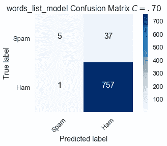通過提高將電子郵件分類為垃圾郵件的標準，13 封正確分類為$C=.50$的垃圾郵件現在被貼錯標簽。 $$ \text{Sensitivity } (C = .70) = \frac{5}{42} \approx .119 \\ \text{Specificity } (C = .70) = \frac{757}{758} \approx .999 $$ 與默認值相比，更高的閾值$C=.70$增加了特異性，但降低了敏感性。 將閾值降低到$C=0.30 美元，這意味著如果概率$F \that \theta（x）$大于.30，我們會將電子郵件$X$標記為垃圾郵件，從而導致以下混淆矩陣： ``` # HIDDEN words_list_predictions = [1 if pred >= .30 else 0 for pred in words_list_prediction_probabilities] low_classification_threshold = confusion_matrix(y_train, words_list_predictions, labels=[1, 0]) plot_confusion_matrix(low_classification_threshold, classes=class_names, title='words_list_model Confusion Matrix $C = .30$') ```  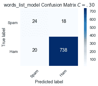通過降低將電子郵件分類為垃圾郵件的標準，6 封錯誤標記為$C=.50$的垃圾郵件現在是正確的。然而，有更多的誤報。 $$ \text{Sensitivity } (C = .30) = \frac{24}{42} \approx .571 \\ \text{Specificity } (C = .30) = \frac{738}{758} \approx .974 $$ 與默認值相比，較低的閾值$C=.30$增加了敏感性，但降低了特異性。 我們通過改變分類閾值來調整模型的敏感性和特異性。盡管我們努力最大限度地提高敏感性和特異性，但從用不同分類閾值創建的混淆矩陣中可以看出，存在一種權衡。敏感性增加導致特異性降低，反之亦然。 ### ROC 曲線 我們可以計算 0 到 1 之間所有分類閾值的敏感性和特異性值，并繪制它們。每個閾值$c$與一對（敏感性、特異性）相關。**ROC（接收器工作特性）曲線**是對這一想法的一個細微修改；它不是繪制（敏感性、特異性）曲線，而是繪制（敏感性、1-特異性）對，其中 1-特異性被定義為假陽性率。 $$ \text{False Positive Rate } = 1 - \frac{TN}{TN + FP} = \frac{TN + FP - TN}{TN + FP} = \frac{FP}{TN + FP} $$ ROC 曲線上的一個點表示與特定閾值相關的靈敏度和假陽性率。 使用 SciKit Learn 的[roc 曲線函數](http://scikit-learn.org/stable/modules/generated/sklearn.metrics.roc_curve.html)計算`words_list_model`的 roc 曲線： ``` from sklearn.metrics import roc_curve words_list_model_probabilities = words_list_model.predict_proba(X_train)[:, 1] false_positive_rate_values, sensitivity_values, thresholds = roc_curve(y_train, words_list_model_probabilities, pos_label=1) ``` ``` # HIDDEN plt.step(false_positive_rate_values, sensitivity_values, color='b', alpha=0.2, where='post') plt.xlabel('False Positive Rate (1 - Specificity)') plt.ylabel('Sensitivity') plt.title('words_list_model ROC Curve') ``` ``` Text(0.5,1,'words_list_model ROC Curve') ```  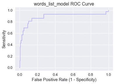注意，當我們在曲線上從左向右移動時，敏感性增加，特異性降低。一般來說，最佳分類閾值對應于高靈敏度和特異性（低假陽性率），因此最好是位于地塊西北角或附近的點。 讓我們來檢查一下圖的四個角： * （0，0）：特異性$=1$，這意味著負類中的所有數據點都被正確標記，但敏感性$=0$，因此模型沒有真正的正性。（0,0）映射到分類閾值$c=1.0$，這與`ham_only`具有相同的效果，因為沒有電子郵件的概率大于$1.0$。 * （1，1）：特異性$=0$，這意味著模型沒有真正的負性，但敏感性$=1$，所以正類中的所有數據點都被正確標記。（1,1）映射到分類閾值$c=0.0$，這與`spam_only`具有相同的效果，因為沒有電子郵件的概率低于$0.0$。 * （0，1）：特異性$=1$和敏感性$=1$，這意味著沒有假陽性或假陰性。具有包含（0，1）的 ROC 曲線的模型具有$C$值，在該值上它是一個完美的分類器！ * （1，0）：特異性.=0$和敏感性.=0$，這意味著沒有真陽性或真陰性。具有包含（1，0）的 ROC 曲線的模型具有$C$值，在該值處它預測每個數據點的錯誤類！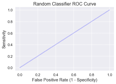 隨機預測類的分類器有一條包含靈敏度和假陽性率相等的所有點的對角 ROC 曲線： ``` # HIDDEN plt.step(np.arange(0, 1, 0.001), np.arange(0, 1, 0.001), color='b', alpha=0.2, where='post') plt.xlabel('False Positive Rate (1 - Specificity)') plt.ylabel('Sensitivity') plt.title('Random Classifier ROC Curve') ``` ``` Text(0.5,1,'Random Classifier ROC Curve') ```  直觀地說，一個隨機分類器預測輸入$x$的概率$p$將導致機會$p$的真正或假正，因此靈敏度和假正率相等。 我們希望分類器的 ROC 曲線高出隨機模型診斷線，這將我們引入 AUC 度量。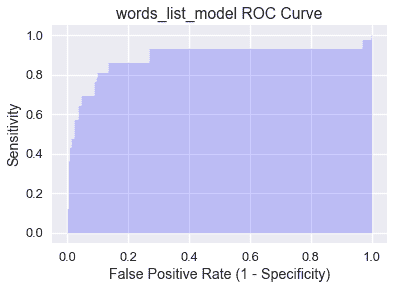 ### AUC[？](#AUC) 曲線下的**面積（auc）**是 roc 曲線下的面積，用作分類器的單個數字性能摘要。下面陰影顯示了`words_list_model`的 AUC，并使用 SciKit Learn 的[AUC 函數](http://scikit-learn.org/stable/modules/generated/sklearn.metrics.roc_auc_score.html#sklearn.metrics.roc_auc_score)進行計算： ``` # HIDDEN plt.fill_between(false_positive_rate_values, sensitivity_values, step='post', alpha=0.2, color='b') plt.xlabel('False Positive Rate (1 - Specificity)') plt.ylabel('Sensitivity') plt.title('words_list_model ROC Curve') ``` ``` Text(0.5,1,'words_list_model ROC Curve') ```  ``` from sklearn.metrics import roc_auc_score roc_auc_score(y_train, words_list_model_probabilities) ``` ``` 0.9057984671441136 ``` AUC 被解釋為分類器將更高的概率分配給真正屬于正類的隨機選擇的數據點，而不是真正屬于負類的隨機選擇的數據點。完美的 AUC 值 1 對應于完美的分類器（ROC 曲線將包含（0，1）。事實上，`words_list_model`的 AUC 為.906 意味著大約 90.6%的時間將垃圾郵件分類為垃圾郵件，而不是將火腿電子郵件分類為垃圾郵件。 經檢驗，隨機分類器的 AUC 為 0.5，盡管這可能由于隨機性而略有變化。一個有效的模型的 AUC 將遠高于`words_list_model`所達到的 0.5。如果模型的 AUC 小于 0.5，那么它的性能會比隨機預測差。 ### 摘要[?](#Summary) AUC 是評估類不平衡數據集模型的重要指標。在對模型進行訓練后，最好生成 ROC 曲線并計算 AUC 以確定下一步。如果 AUC 足夠高，使用 ROC 曲線確定最佳分類閾值。但是，如果 AUC 不滿意，考慮進一步進行 EDA 和特征選擇以改進模型。