# L1 正則化：LASSO 回歸 > 原文：[https://www.textbook.ds100.org/ch/16/reg_lasso.html](https://www.textbook.ds100.org/ch/16/reg_lasso.html) ``` # HIDDEN # Clear previously defined variables %reset -f # Set directory for data loading to work properly import os os.chdir(os.path.expanduser('~/notebooks/16')) ``` ``` # HIDDEN import warnings # Ignore numpy dtype warnings. These warnings are caused by an interaction # between numpy and Cython and can be safely ignored. # Reference: https://stackoverflow.com/a/40846742 warnings.filterwarnings("ignore", message="numpy.dtype size changed") warnings.filterwarnings("ignore", message="numpy.ufunc size changed") import numpy as np import matplotlib.pyplot as plt import pandas as pd import seaborn as sns %matplotlib inline import ipywidgets as widgets from ipywidgets import interact, interactive, fixed, interact_manual import nbinteract as nbi sns.set() sns.set_context('talk') np.set_printoptions(threshold=20, precision=2, suppress=True) pd.options.display.max_rows = 7 pd.options.display.max_columns = 8 pd.set_option('precision', 2) # This option stops scientific notation for pandas # pd.set_option('display.float_format', '{:.2f}'.format) ``` ``` # HIDDEN def df_interact(df, nrows=7, ncols=7): ''' Outputs sliders that show rows and columns of df ''' def peek(row=0, col=0): return df.iloc[row:row + nrows, col:col + ncols] if len(df.columns) <= ncols: interact(peek, row=(0, len(df) - nrows, nrows), col=fixed(0)) else: interact(peek, row=(0, len(df) - nrows, nrows), col=(0, len(df.columns) - ncols)) print('({} rows, {} columns) total'.format(df.shape[0], df.shape[1])) ``` ``` # HIDDEN df = pd.read_csv('water_large.csv') ``` ``` # HIDDEN from collections import namedtuple Curve = namedtuple('Curve', ['xs', 'ys']) def flatten(seq): return [item for subseq in seq for item in subseq] def make_curve(clf, x_start=-50, x_end=50): xs = np.linspace(x_start, x_end, num=100) ys = clf.predict(xs.reshape(-1, 1)) return Curve(xs, ys) def plot_data(df=df, ax=plt, **kwargs): ax.scatter(df.iloc[:, 0], df.iloc[:, 1], s=50, **kwargs) def plot_curve(curve, ax=plt, **kwargs): ax.plot(curve.xs, curve.ys, **kwargs) def plot_curves(curves, cols=2, labels=None): if labels is None: labels = [f'Deg {deg} poly' for deg in degrees] rows = int(np.ceil(len(curves) / cols)) fig, axes = plt.subplots(rows, cols, figsize=(10, 8), sharex=True, sharey=True) for ax, curve, label in zip(flatten(axes), curves, labels): plot_data(ax=ax, label='Training data') plot_curve(curve, ax=ax, label=label) ax.set_ylim(-5e10, 170e10) ax.legend() # add a big axes, hide frame fig.add_subplot(111, frameon=False) # hide tick and tick label of the big axes plt.tick_params(labelcolor='none', top='off', bottom='off', left='off', right='off') plt.grid(False) plt.title('Polynomial Regression') plt.xlabel('Water Level Change (m)') plt.ylabel('Water Flow (Liters)') plt.tight_layout() ``` ``` # HIDDEN def coefs(clf): reg = clf.named_steps['reg'] return np.append(reg.intercept_, reg.coef_) def coef_table(clf): vals = coefs(clf) return (pd.DataFrame({'Coefficient Value': vals}) .rename_axis('degree')) ``` ``` # HIDDEN X = df.iloc[:, [0]].as_matrix() y = df.iloc[:, 1].as_matrix() degrees = [1, 2, 8, 12] clfs = [Pipeline([('poly', PolynomialFeatures(degree=deg, include_bias=False)), ('reg', LinearRegression())]) .fit(X, y) for deg in degrees] curves = [make_curve(clf) for clf in clfs] alphas = [0.1, 1.0, 10.0] ridge_clfs = [Pipeline([('poly', PolynomialFeatures(degree=deg, include_bias=False)), ('reg', RidgeCV(alphas=alphas, normalize=True))]) .fit(X, y) for deg in degrees] ridge_curves = [make_curve(clf) for clf in ridge_clfs] lasso_clfs = [Pipeline([('poly', PolynomialFeatures(degree=deg, include_bias=False)), ('reg', LassoCV(normalize=True, precompute=True, tol=0.001))]) .fit(X, y) for deg in degrees] lasso_curves = [make_curve(clf) for clf in lasso_clfs] ``` 在本節中，我們將介紹$L_1$正則化，這是另一種對特性選擇有用的正則化技術。 我們首先簡要回顧線性回歸的$L_2$正則化。我們使用模型： $$ f_\hat{\theta}(x) = \hat{\theta} \cdot x $$ 我們通過用一個額外的正則化項最小化均方誤差成本函數來擬合模型： $$ \begin{aligned} L(\hat{\theta}, X, y) &= \frac{1}{n} \sum_{i}(y_i - f_\hat{\theta} (X_i))^2 + \lambda \sum_{j = 1}^{p} \hat{\theta_j}^2 \end{aligned} $$ 在上述定義中，$x$表示$n 乘以 p$數據矩陣，$x$表示$x$的一行，$y$表示觀察到的結果，$hat \theta$表示模型權重，$lambda$表示正則化參數。 ## 一級規范化定義 要將$L_1$正則化添加到模型中，我們修改上面的成本函數： $$ \begin{aligned} L(\hat{\theta}, X, y) &= \frac{1}{n} \sum_{i}(y_i - f_\hat{\theta} (X_i))^2 + \lambda \sum_{j = 1}^{p} |\hat{\theta_j}| \end{aligned} $$ 注意，這兩個成本函數的正則化條件不同。$L_1$正則化懲罰絕對權重值之和，而不是平方值之和。 在線性模型和均方誤差成本函數中使用$L_1$正則化，通常也被稱為**lasso 回歸**。（lasso 代表最小絕對收縮和選擇運算符。） ## 比較 lasso 和 ridge 回歸 為了進行 lasso 回歸，我們使用了`scikit-learn`便利的[`LassoCV`](http://scikit-learn.org/stable/modules/generated/sklearn.linear_model.LassoCV.html)分類器，它是執行交叉驗證以選擇正則化參數的[`Lasso`](http://scikit-learn.org/stable/modules/generated/sklearn.linear_model.Lasso.html)分類器的一個版本。下面，我們顯示了我們的水位變化和大壩流出水量的數據集。 ``` # HIDDEN df ``` | | 水位變化 | 水流 | | --- | --- | --- | | 零 | -15 | 60422330445.52 號 | | --- | --- | --- | | 1 個 | -27.15 | 33214896575.60 元 | | --- | --- | --- | | 二 | 三十六點一九 | 972706380901.06 | | --- | --- | --- | | …… | …… | ... | | --- | --- | --- | | 20 個 | 七點零九 | 236352046523.78 個 | | --- | --- | --- | | 21 歲 | 四十六點二八 | 149425638186.73 | | --- | --- | --- | | 二十二 | 十四點六一 | 378146284247.97 美元 | | --- | --- | --- | 23 行×2 列 由于該過程幾乎與使用上一節中的`RidgeCV`分類器相同，因此我們省略了代碼，而是顯示下面的基階 12 多項式、嶺回歸和 lasso 回歸模型預測。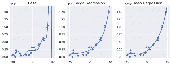 ``` # HIDDEN fig = plt.figure(figsize=(10, 4)) plt.subplot(131) plot_data() plot_curve(curves[3]) plt.title('Base') plt.ylim(-5e10, 170e10) plt.subplot(132) plot_data() plot_curve(ridge_curves[3]) plt.title('Ridge Regression') plt.ylim(-5e10, 170e10) plt.subplot(133) plot_data() plot_curve(lasso_curves[3]) plt.title('Lasso Regression') plt.ylim(-5e10, 170e10) plt.tight_layout() ```  我們可以看到，兩個正則化模型的方差都小于基度 12 多項式。乍一看，使用$L_2$和$L_1$正則化可以生成幾乎相同的模型。然而，比較嶺回歸和套索回歸的系數，可以發現兩種正則化類型之間最顯著的差異：套索回歸模型將若干模型權重設置為零。 ``` # HIDDEN ridge = coef_table(ridge_clfs[3]).rename(columns={'Coefficient Value': 'Ridge'}) lasso = coef_table(lasso_clfs[3]).rename(columns={'Coefficient Value': 'Lasso'}) pd.options.display.max_rows = 20 pd.set_option('display.float_format', '{:.10f}'.format) display(ridge.join(lasso)) pd.options.display.max_rows = 7 pd.set_option('display.float_format', '{:.2f}'.format) ``` | | 山脊 | 套索 | | --- | --- | --- | | 度 | | | | --- | --- | --- | | 0 | 221303288116.2275085449 | 198212062407.2835693359 | | --- | --- | --- | | 1 | 6953405307.7653837204 | 9655088668.0876655579 | | --- | --- | --- | | 2 | 142621063.9297277331 | 198852674.1646585464 | | --- | --- | --- | | 三 | 1893283.0567885502 年 | 0.000000 萬 | | --- | --- | --- | | 四 | 38202.1520293704 號 | 34434.3458919188 年 | | --- | --- | --- | | 5 個 | 484.4262914111 號 | 975.6965959434 | | --- | --- | --- | | 六 | 8.1525126516 | 0.0000000000 | | --- | --- | --- | | 七 | 0.1197232472 | 0.0887942172 個 | | --- | --- | --- | | 8 個 | 0.0012506185 | 0.0000000000 | | --- | --- | --- | | 九 | 0.0000289599 元 | 0.0000000000 | | --- | --- | --- | | 10 個 | -0.000000000 萬 4 | 0.0000000000 | | --- | --- | --- | | 11 個 | 0.0000000069 美元 | 0.0000000000 | | --- | --- | --- | | 12 個 | -0.00000000001 美元 | -0.000000 萬 | | --- | --- | --- | 如果您原諒上面的詳細輸出，您將注意到脊回歸會導致所有多項式特性的非零權重。另一方面，套索回歸為七個特征生成了 0 的權重。 換句話說，當進行預測時，套索回歸模型完全拋棄了大部分特征。盡管如此，上面的曲線圖顯示，與嶺回歸模型相比，lasso 回歸模型將做出幾乎相同的預測。 ## 使用 lasso 回歸的功能選擇[?](#Feature-Selection-with-Lasso-Regression) lasso 回歸執行**特征選擇**——它在擬合模型參數時丟棄原始特征的子集。這在處理具有許多特性的高維數據時特別有用。一個只使用少數特征進行預測的模型比一個需要大量計算的模型運行得更快。由于不需要的特征傾向于在不降低偏差的情況下增加模型方差，我們有時可以通過使用 lasso 回歸選擇要使用的特征子集來提高其他模型的精度。 ## 實踐中的套索與山脊 如果我們的目標僅僅是達到最高的預測精度，我們可以嘗試兩種類型的正則化，并使用交叉驗證在這兩種類型之間進行選擇。 有時我們更喜歡一種類型的正則化而不是另一種，因為它更接近于我們正在處理的領域。例如，如果知道我們試圖從許多小因素模擬結果的現象，我們可能更喜歡嶺回歸，因為它不會丟棄這些因素。另一方面，一些具有高度影響力的特征導致了一些結果。在這些情況下，我們更喜歡 lasso 回歸，因為它將丟棄不需要的特性。 ## 摘要[?](#Summary) 使用$L_1$正則化，如$L_2$正則化，可以通過懲罰大型模型權重來調整模型偏差和方差。$L_1$最小二乘線性回歸的正則化也被更常見的名稱 lasso 回歸所知。套索回歸也可用于執行特征選擇，因為它丟棄了不重要的特征。