# 線性回歸的自舉（真系數的推斷） > 原文：[https://www.bookbookmark.ds100.org/ch/18/hyp_regression.html](https://www.bookbookmark.ds100.org/ch/18/hyp_regression.html) ``` # HIDDEN # Clear previously defined variables %reset -f # Set directory for data loading to work properly import os os.chdir(os.path.expanduser('~/notebooks/18')) ``` ``` # HIDDEN import warnings # Ignore numpy dtype warnings. These warnings are caused by an interaction # between numpy and Cython and can be safely ignored. # Reference: https://stackoverflow.com/a/40846742 warnings.filterwarnings("ignore", message="numpy.dtype size changed") warnings.filterwarnings("ignore", message="numpy.ufunc size changed") import numpy as np import matplotlib.pyplot as plt import pandas as pd import seaborn as sns %matplotlib inline import ipywidgets as widgets from ipywidgets import interact, interactive, fixed, interact_manual import nbinteract as nbi sns.set() sns.set_context('talk') np.set_printoptions(threshold=20, precision=2, suppress=True) pd.options.display.max_rows = 7 pd.options.display.max_columns = 8 pd.set_option('precision', 2) # This option stops scientific notation for pandas # pd.set_option('display.float_format', '{:.2f}'.format) ``` 回想一下，在線性回歸中，我們擬合了如下形式的模型：$\ begin aligned f \ theta（x）=\hat \ theta+hat \ theta x u 1+\ldots+\hat \ theta x u p\end aligned$$ 我們想推斷模型的真實系數。由于$\hat \theta 0，$\hat \theta，$\ldots$\hat \theta p 是根據我們的培訓數據/觀察結果而變化的估計量，我們想了解我們的估計系數與真實系數的比較情況。bootstrapping 是一種統計推斷的非參數方法，它為我們的參數提供了標準誤差和置信區間。 讓我們來看一個如何在線性回歸中使用引導方法的例子。 ### 數據[?](#The-Data) 奧蒂斯·達德利·鄧肯是一位定量社會學家，對衡量不同職業的聲望水平感興趣。在 1947 年的國家意見研究中心（Norc）調查中，只有 90 個職業被評為他們的聲望水平。鄧肯希望通過使用 1950 年人口普查記錄的每個職業的收入和教育數據來“填寫”未分級職業的聲望分數。當把北卡羅來納州的數據與 1950 年的人口普查數據相結合時，只有 45 個職業可以匹配。最后，鄧肯的目標是建立一個模型，用不同的特征來解釋威望；使用這個模型，人們可以預測在挪威國家石油公司調查中沒有記錄的其他職業的威望。 鄧肯數據集是一個隨機樣本，其中包含 1950 年美國 45 個職業的聲望和其他特征的信息。變量包括： `occupation`表示職業/頭銜的類型。 `income`表示收入超過 3500 美元的職業在職人員的百分比。 `education`代表 1950 年美國人口普查中在職者中高中畢業生的百分比。 `prestige`表示在一項調查中，被調查者在聲望上認為某一職業“好”或“優秀”的百分比。 ``` duncan = pd.read_csv('duncan.csv').loc[:, ["occupation", "income", "education", "prestige"]] duncan ``` | | 職業 | 收入 | 教育 | 聲望 | | --- | --- | --- | --- | --- | | 零 | 會計 | 六十二 | 86 歲 | 八十二 | | --- | --- | --- | --- | --- | | 1 個 | 飛行員 | 七十二 | 七十六 | 八十三 | | --- | --- | --- | --- | --- | | 二 | 建筑師 | 75 歲 | 92 歲 | 九十 | | --- | --- | --- | --- | --- | | …… | …… | ... | ... | ... 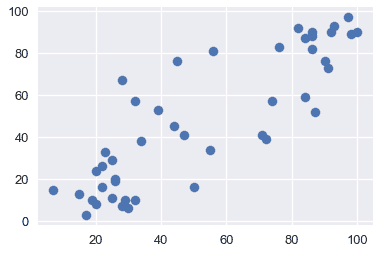| | --- | --- | --- | --- | --- | | 42 歲 | 看門人 | 七 | 20 個 | 8 個 | | --- | --- | --- | --- | --- | | 四十三 | 警察 | 34 歲 | 47 歲 | 四十一 | | --- | --- | --- | --- | --- | | 四十四 | 服務員 | 8 | 三十二 | 10 個 | | --- | --- | --- | --- | --- | 45 行×4 列 通過可視化來探索數據通常是一個好主意，以便了解變量之間的關系。下面，我們將看到收入、教育和聲望之間的關系。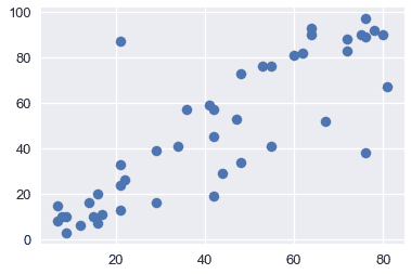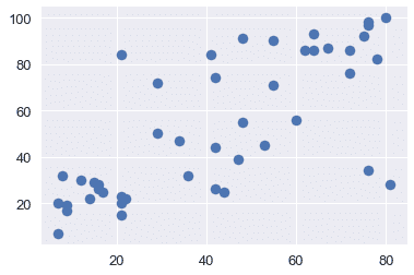 ``` plt.scatter(x=duncan["education"], y=duncan["prestige"]) ``` ``` <matplotlib.collections.PathCollection at 0x1a1cf2cd30> ```  ``` plt.scatter(x=duncan["income"], y=duncan["prestige"]) ``` ``` <matplotlib.collections.PathCollection at 0x1a1d0224e0> ```  ``` plt.scatter(x=duncan["income"], y=duncan["education"]) ``` ``` <matplotlib.collections.PathCollection at 0x1a1d0de5f8> ```  從上面的圖中，我們看到教育和收入與聲望呈正相關；因此，這兩個變量可能有助于解釋聲望。讓我們用這些解釋變量擬合一個線性模型來解釋聲望。 ### 擬合模型[?](#Fitting-the-model) 我們將采用以下模型來解釋職業聲望作為收入和教育的線性函數： $$\開始對齊\文本 tt 聲望 _i=\theta_0^* * \ theta ^*\cdot\texttt 收入 u i * \ theta 教育^*\cdot\texttt 教育 u i * \ varepsilon_i \結束對齊$$ 為了適應這個模型，我們將定義設計矩陣（x）和響應變量（y）： ``` X = duncan.loc[:, ["income", "education"]] X.head() ``` | | income | education | | --- | --- | --- | | 0 | 62 | 86 | | --- | --- | --- | | 1 | 72 | 76 | | --- | --- | --- | | 2 | 75 | 92 | | --- | --- | --- | | 三 | 55 歲 | 90 | | --- | --- | --- | | 四 | 六十四 | 86 | | --- | --- | --- | ``` y = duncan.loc[:, "prestige"] y.head() ``` ``` 0 82 1 83 2 90 3 76 4 90 Name: prestige, dtype: int64 ``` 下面，我們擬合我們的線性模型，并在模型與數據相匹配后，打印出模型的所有系數（從上面的方程式中）。注意，這些是我們的樣本系數。 ``` import sklearn.linear_model as lm linear_model = lm.LinearRegression() linear_model.fit(X, y) print(""" intercept: %.2f income: %.2f education: %.2f """ % (tuple([linear_model.intercept_]) + tuple(linear_model.coef_))) ``` ``` intercept: -6.06 income: 0.60 education: 0.55 ``` 上面的系數給出了真實系數的估計。但是，如果我們的樣本數據是不同的，我們將使我們的模型適合不同的數據，導致這些系數是不同的。我們想探討一下，我們的系數可能使用了引導方法。 在我們的引導方法和分析中，我們將關注教育系數。我們希望探討聲譽與教育之間的部分關系，即保持收入不變（而不是聲譽與教育之間的邊際關系，而忽略收入）。偏回歸系數$\widehat \theta_uxttet education$說明了我們數據中聲望和教育之間的部分關系。 ### 引導觀察結果[?](#Bootstrapping-the-Observations) 在這種方法中，我們將對$（x_i，y_i）$作為樣本，因此我們通過從這些對中進行替換采樣來構造引導重新采樣： $$\ begin aligned（x_i^*，y_i^*）=（x_i，y_i），\text 其中 i=1，點，n \ text 隨機均勻采樣。\ end aligned$$ 換句話說，我們從我們的數據點用替換的方法對 n 個觀測進行采樣；這是我們的引導樣本。然后我們將一個新的線性回歸模型擬合到這個樣本數據中，并記錄教育系數$\tilde\theta\texttt education$；這個系數是我們的引導統計。 #### $\tilde\theta\texttt 教育$[？](#Bootstrap-Sampling-Distribution-of-$\tilde\theta_\texttt{education}$)的引導抽樣分布 ``` def simple_resample(n): return(np.random.randint(low = 0, high = n, size = n)) def bootstrap(boot_pop, statistic, resample = simple_resample, replicates = 10000): n = len(boot_pop) resample_estimates = np.array([statistic(boot_pop[resample(n)]) for _ in range(replicates)]) return resample_estimates ``` ``` def educ_coeff(data_array): X = data_array[:, 1:] y = data_array[:, 0] linear_model = lm.LinearRegression() model = linear_model.fit(X, y) theta_educ = model.coef_[1] return theta_educ data_array = duncan.loc[:, ["prestige", "income", "education"]].values theta_hat_sampling = bootstrap(data_array, educ_coeff) ``` ``` plt.figure(figsize = (7, 5)) plt.hist(theta_hat_sampling, bins = 30, normed = True) plt.xlabel("$\\tilde{\\theta}_{educ}$ Values") plt.ylabel("Proportion per Unit") plt.title("Bootstrap Sampling Distribution of $\\tilde{\\theta}_{educ}$ (Nonparametric)"); plt.show() ```  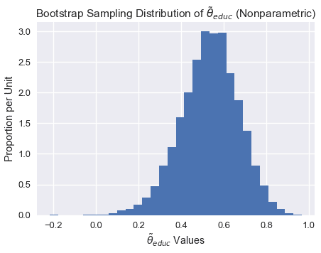注意上面的采樣分布是如何稍微向左傾斜的。 #### 估算真系數 雖然我們不能直接測量$\theta^*u \texttt education$我們可以使用引導置信區間來解釋樣本回歸系數$\widehat\theta \texttt education 的可變性。下面，我們使用 bootstrap percentile 方法為真系數$\theta^*\texttt education 構建一個大約 95%的置信區間。置信區間從 2.5%擴展到 10000 個自舉系數的 97.5%。 ``` left_confidence_interval_endpoint = np.percentile(theta_hat_sampling, 2.5) right_confidence_interval_endpoint = np.percentile(theta_hat_sampling, 97.5) left_confidence_interval_endpoint, right_confidence_interval_endpoint ``` ``` (0.24714198882974781, 0.78293602739856061) ``` 從上述置信區間，我們可以相當確定，真實系數介于 0.236 和 0.775 之間。 #### 利用正態理論的置信區間 我們也可以建立基于正態理論的置信區間。由于$\widehat\theta educ 值呈正態分布，我們可以通過計算以下內容來構造置信區間： $$\begin aligned[\widehat\theta-z \frac \alpha 2 se（\theta ^*），\widehat\theta+z \frac \alpha 2 se（\theta ^*）]\end aligned$$ 其中，$se（\theta^*）$是引導系數的標準誤差，$z$是一個常數，$widehat\theta$是我們的樣本系數。注意$Z$根據我們構建的區間的置信水平而變化。由于我們正在建立一個 95%的置信區間，我們將使用 1.96。 ``` # We will use the statsmodels library in order to find the standard error of the coefficients import statsmodels.api as sm ols = sm.OLS(y, X) ols_result = ols.fit() # Now you have at your disposition several error estimates, e.g. ols_result.HC0_se ``` ``` income 0.15 education 0.12 dtype: float64 ``` ``` left_confidence_interval_endpoint_normal = 0.55 - (1.96*0.12) right_confidence_interval_endpoint_normal = 0.55 + (1.96*0.12) left_confidence_interval_endpoint_normal, right_confidence_interval_endpoint_normal ``` ``` (0.3148000000000001, 0.7852) ``` **觀察值：**注意使用正態理論的置信區間比使用百分位法的置信區間窄，特別是在區間的左邊。 我們不會詳細討論正常理論置信區間，但如果您想了解更多信息，請參閱 x。 #### 真系數可以是 0 嗎？[?](#Could-the-true-coefficient-be-0?) 雖然我們觀察到教育和聲望之間存在正的部分關系（從 0.55 系數開始），但如果真正的系數是 0，而教育和聲望之間沒有部分關系呢？在這種情況下，我們觀察到的關聯僅僅是由于在獲得構成我們樣本的點時的變化。 為了正式檢驗教育與聲望之間的部分關系是否真實，我們要檢驗以下假設： **虛假設**真偏系數為 0。 **替代假設。**真正的分項系數不是 0。 由于我們已經為真系數建立了 95%的置信區間，我們只需要看看 0 是否在這個區間內。請注意，0 不在上述置信區間內；因此，我們有足夠的證據來拒絕無效假設。 如果真系數的置信區間確實包含 0，那么我們就沒有足夠的證據來拒絕無效假設。在這種情況下，觀察到的系數$\widehat\theta \textt education$可能是假的。 #### 方法 1 引導反射 為了建立系數$\widehat\theta \texttt education 的抽樣分布，并構造真系數的置信區間，我們直接對觀測結果進行了重采樣，并在引導樣本上擬合了新的回歸模型。此方法將回歸量$x_i$隱式地視為隨機的，而不是固定的。 在某些情況下，我們可能希望將$x_i$視為固定值（例如，如果數據來自實驗設計）。如果解釋變量被控制，或者解釋變量的值被實驗者設置，那么我們可以考慮下面的替代引導方法。 ### 備選方案：引導殘差[?](#Alternative:-Bootstrapping-the-Residuals) 線性回歸中假設檢驗的另一種方法是自舉殘差。這種方法有許多基本假設，在實踐中使用頻率較低。在這種方法中，我們將 _ 殘差 _$e_i：=y_i-x_i \widehat \beta$作為我們的樣本，因此我們通過用這些殘差替換的樣本來構造引導重采樣。一旦我們構造了每個引導樣本，我們就可以使用這些殘差計算新的擬合值。然后，我們將這些新的 y 值回歸到固定的 x 值上，得到自舉回歸系數。 為了更清楚地說明，讓我們將此方法分解為以下步驟： 1. 估計原始樣本的回歸系數，并計算每個觀測值的擬合值$\widehat y$和殘差$e_i$。 2. 選擇殘差的引導樣本；我們將這些引導殘差表示為$\tilde e_1、\tilde e_2、\dots\tilde e_n$。然后，通過計算$\widehat y+\tilde e_i$計算引導的$\tilde y_i$值，其中擬合值$\widehat y_i=x_i\widehat\beta$從原始回歸中獲得。 3. 在固定的$x$值上對引導的$\tilde y_i$值進行回歸，以獲得引導回歸系數$\tilde\theta$。 4. 重復第二步和第三步數次，以獲得幾個引導回歸系數$\tilde\theta_1、\tilde\theta_2、\dots\tilde\theta_n$。這些可以用來計算引導標準錯誤和置信區間。 #### Estimating the True Coefficients[?](#Estimating-the-True-Coefficients) 既然我們已經有了自舉回歸系數，我們可以使用與以前相同的技術構造一個置信區間。我們將把這個留作練習。 #### 引導殘差反射[？](#Bootstrapping-the-Residuals-Reflection) 讓我們考慮一下這個方法。通過將重新取樣的殘差隨機重新附加到確定的值，此過程隱式地假定錯誤分布相同。更具體地說，該方法假定輸入$x_i$的所有值的回歸曲線周圍的波動分布是相同的。這是一個缺點，因為真正的錯誤可能有不恒定的方差；這種現象被稱為異方差。 雖然這種方法沒有對誤差分布的形狀做任何假設，但它隱式地假定模型的函數形式是正確的。通過依賴模型來創建每個引導樣本，我們假設模型結構是適當的。 ## 摘要[?](#Summary) 在本節中，我們將重點介紹線性回歸設置中使用的引導技術。 一般來說，引導觀察通常用于引導。該方法通常比其他技術更為穩健，因為它所做的基本假設更少；例如，如果擬合了錯誤的模型，則該方法仍將生成相關參數的適當抽樣分布。 我們還強調了另一種方法，它有幾個缺點。當我們希望將我們的觀察值$x$視為固定值時，可以使用引導殘差。請注意，應該謹慎使用此方法，因為它對模型的錯誤和形式進行了額外的假設。