# 線性回歸案例研究 > 原文：[https://www.bookbookmark.ds100.org/ch/13/linear_case_study.html](https://www.bookbookmark.ds100.org/ch/13/linear_case_study.html) ``` # HIDDEN # Clear previously defined variables %reset -f # Set directory for data loading to work properly import os os.chdir(os.path.expanduser('~/notebooks/13')) ``` ``` # HIDDEN import warnings # Ignore numpy dtype warnings. These warnings are caused by an interaction # between numpy and Cython and can be safely ignored. # Reference: https://stackoverflow.com/a/40846742 warnings.filterwarnings("ignore", message="numpy.dtype size changed") warnings.filterwarnings("ignore", message="numpy.ufunc size changed") import numpy as np import matplotlib.pyplot as plt import pandas as pd import seaborn as sns %matplotlib inline import ipywidgets as widgets from ipywidgets import interact, interactive, fixed, interact_manual import nbinteract as nbi sns.set() sns.set_context('talk') np.set_printoptions(threshold=20, precision=2, suppress=True) pd.options.display.max_rows = 7 pd.options.display.max_columns = 8 pd.set_option('precision', 2) # This option stops scientific notation for pandas # pd.set_option('display.float_format', '{:.2f}'.format) ``` ``` # HIDDEN from scipy.optimize import minimize as sci_min def minimize(cost_fn, grad_cost_fn, X, y, progress=True): ''' Uses scipy.minimize to minimize cost_fn using a form of gradient descent. ''' theta = np.zeros(X.shape[1]) iters = 0 def objective(theta): return cost_fn(theta, X, y) def gradient(theta): return grad_cost_fn(theta, X, y) def print_theta(theta): nonlocal iters if progress and iters % progress == 0: print(f'theta: {theta} | cost: {cost_fn(theta, X, y):.2f}') iters += 1 print_theta(theta) return sci_min( objective, theta, method='BFGS', jac=gradient, callback=print_theta, tol=1e-7 ).x ``` 在本節中，我們將執行一個將線性回歸模型應用到數據集的端到端案例研究。我們將使用的數據集具有各種屬性，例如驢的長度和周長。 我們的任務是用線性回歸預測一頭驢的體重。 ## 初步數據概述 我們將從讀取數據集開始，并快速查看其內容。 ``` donkeys = pd.read_csv("donkeys.csv") donkeys.head() ``` | | 基站控制系統 | 年齡 | 性 | …… | 高度 | 重量 | 權重 alt | | --- | --- | --- | --- | --- | --- | --- | --- | | 零 | 三 | lt；2 | 種馬 | …… | 九十 | 七十七 | 南 | | --- | --- | --- | --- | --- | --- | --- | --- | | 1 個 | 2.5 條 | &lt;2 | stallion | ... | 94 歲 | 100 個 | NaN | | --- | --- | --- | --- | --- | --- | --- | --- | | 二 | 1.5 條 | &lt;2 | stallion | ... | 九十五 | 七十四 | NaN | | --- | --- | --- | --- | --- | --- | --- | --- | | 三 | 3.0 | &lt;2 | 女性的 | ... | 九十六 | 一百一十六 | NaN | | --- | --- | --- | --- | --- | --- | --- | --- | | 四 | 2.5 | &lt;2 | female | ... | 91 歲 | 91 | NaN | | --- | --- | --- | --- | --- | --- | --- | --- | 5 行×8 列 通過查看數據集的維度，查看 _ 我們有多少 _ 數據總是一個好主意。如果我們有大量的觀察結果，打印出整個數據幀可能會使我們的筆記本崩潰。 ``` donkeys.shape ``` ``` (544, 8) ``` 數據集相對較小，只有 544 行觀察值和 8 列。讓我們看看哪些列對我們可用。 ``` donkeys.columns.values ``` ``` array(['BCS', 'Age', 'Sex', 'Length', 'Girth', 'Height', 'Weight', 'WeightAlt'], dtype=object) ``` 對數據的良好理解可以指導我們的分析，因此我們應該理解這些列中的每一列代表什么。其中一些列是不言自明的，但其他的則需要更多的解釋： * 【HTG0】：身體狀況評分（身體健康等級） * 【HTG0】：驢中間的測量 * 【HTG0】：第二次稱重（我們數據中 31 頭驢稱重兩次，以檢查天平的精度） 確定哪些變量是定量的，哪些是分類的也是一個好主意。 定量：【HTG0】、【HTG1】、【HTG2】、【HTG3】、【HTG4】 分類：【HTG0】、【HTG1】、【HTG2】 ## 數據清理 在本節中，我們將檢查數據中是否存在需要處理的異常情況。 通過更仔細地檢查`WeightAlt`，我們可以通過測量兩種不同稱重之間的差異并繪制它們來確保磅秤的準確度。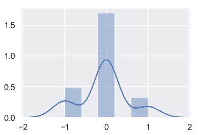 ``` difference = donkeys['WeightAlt'] - donkeys['Weight'] sns.distplot(difference.dropna()); ```  測量值都在 1 公斤以內，這似乎是合理的。 接下來，我們可以查找可能指示錯誤或其他問題的異常值。我們可以使用分位數函數來檢測異常值。 ``` donkeys.quantile([0.005, 0.995]) ``` | | BCS | 長度 | 周長 | Height | Weight | WeightAlt | | --- | --- | --- | --- | --- | --- | --- | | 零點零零五 | 1.5 | 七十一點一四五 | 九十 | 八十九 | 七十一點七一五 | 九十八點七五 | | --- | --- | --- | --- | --- | --- | --- | | 零點九九五 | 四 | 111.000 個 | 131.285 美元 | 一百一十二 | 214.000 美元 | 一百九十二點八零 | | --- | --- | --- | --- | --- | --- | --- | 對于這些數值列中的每一列，我們可以查看哪些行位于這些分位數之外，以及它們所具有的值。考慮到我們希望我們的模型只適用于健康和成熟的驢。 首先，讓我們看看`BCS`列。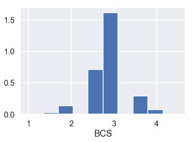 ``` donkeys[(donkeys['BCS'] < 1.5) | (donkeys['BCS'] > 4)]['BCS'] ``` ``` 291 4.5 445 1.0 Name: BCS, dtype: float64 ``` 還可以查看`BCS`的條形圖： ``` plt.hist(donkeys['BCS'], density=True) plt.xlabel('BCS'); ```  考慮到`BCS`是一頭驢健康的標志，1 的`BCS`代表一頭極度消瘦的驢，4.5 的`BCS`代表一頭超重的驢。同樣看一下條形碼，似乎只有兩頭驢有這樣的邊遠值（htg3）。這樣，我們就把這兩只驢移走了。 * * * 現在，讓我們來看一下`Length`、`Girth`和`Height`。 ``` donkeys[(donkeys['Length'] < 71.145) | (donkeys['Length'] > 111)]['Length'] ``` ``` 8 46 22 68 26 69 216 112 Name: Length, dtype: int64 ``` ``` donkeys[(donkeys['Girth'] < 90) | (donkeys['Girth'] > 131.285)]['Girth'] ``` ``` 8 66 239 132 283 134 523 134 Name: Girth, dtype: int64 ``` ``` donkeys[(donkeys['Height'] < 89) | (donkeys['Height'] > 112)]['Height'] ``` ``` 8 71 22 86 244 113 523 116 Name: Height, dtype: int64 ``` 對于這三列，第 8 行中的驢的值似乎比截止值小得多，而其他異常驢則接近截止值，可能不需要移除。 * * * 最后，讓我們來看一下`Weight`。 ``` donkeys[(donkeys['Weight'] < 71.715) | (donkeys['Weight'] > 214)]['Weight'] ``` ``` 8 27 26 65 50 71 291 227 523 230 Name: Weight, dtype: int64 ``` 列表中的前 2 頭和最后 2 頭驢與截止日期相差甚遠，最有可能被移除。中間的驢可以包括在內。 * * * 由于`WeightAlt`與`Weight`密切對應，因此我們跳過檢查此列是否有異常。總結我們所學到的，下面是我們如何過濾我們的驢： * 保持驢子和`BCS`在 1.5 和 4 范圍內 * 把驢子和`Weight`放在 71 到 214 之間 ``` donkeys_c = donkeys[(donkeys['BCS'] >= 1.5) & (donkeys['BCS'] <= 4) & (donkeys['Weight'] >= 71) & (donkeys['Weight'] <= 214)] ``` ## 列車試驗段 在進行數據分析之前，我們將數據分成 80/20 個部分，使用 80%的數據來培訓模型，并留出 20%用于評估模型。 ``` X_train, X_test, y_train, y_test = train_test_split(donkeys_c.drop(['Weight'], axis=1), donkeys_c['Weight'], test_size=0.2, random_state=42) X_train.shape, X_test.shape ``` ``` ((431, 7), (108, 7)) ``` 讓我們還創建一個函數來評估對測試集的預測。我們用均方誤差。 ``` def mse_test_set(predictions): return float(np.sum((predictions - y_test) ** 2)) ``` ## 探索性數據分析與可視化 像往常一樣，我們將在嘗試將模型與之匹配之前探索我們的數據。 首先，我們將用箱線圖檢查分類變量。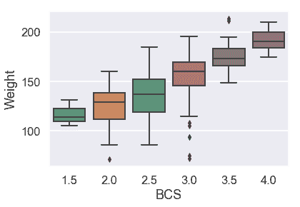 ``` # HIDDEN sns.boxplot(x=X_train['BCS'], y=y_train); ```  似乎體重中位數隨 BCS 增加而增加，但不是線性增加。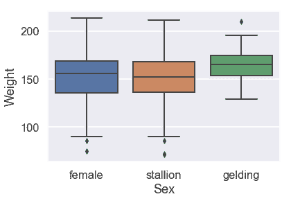 ``` # HIDDEN sns.boxplot(x=X_train['Sex'], y=y_train, order = ['female', 'stallion', 'gelding']); ```  看來驢的性別似乎并沒有引起體重的很大差異。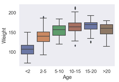 ``` # HIDDEN sns.boxplot(x=X_train['Age'], y=y_train, order = ['<2', '2-5', '5-10', '10-15', '15-20', '>20']); ```  對于 5 歲以上的驢，體重分布沒有太大差異。 現在，讓我們來看看定量變量。我們可以根據目標變量繪制它們中的每一個。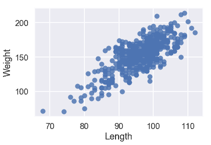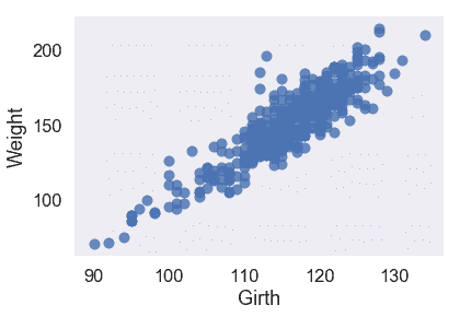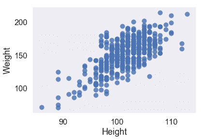 ``` # HIDDEN X_train['Weight'] = y_train sns.regplot('Length', 'Weight', X_train, fit_reg=False); ```  ``` # HIDDEN sns.regplot('Girth', 'Weight', X_train, fit_reg=False); ```  ``` # HIDDEN sns.regplot('Height', 'Weight', X_train, fit_reg=False); ```  我們的三個定量特征都與目標變量`Weight`呈線性關系，因此我們不必對輸入數據執行任何轉換。 看看我們的特性是否是線性的也是一個好主意。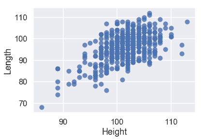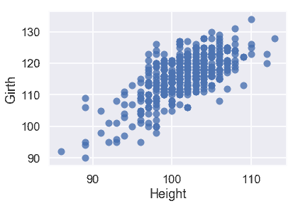我們在下面繪制兩個圖： ``` # HIDDEN sns.regplot('Height', 'Length', X_train, fit_reg=False); ```  ``` # HIDDEN sns.regplot('Height', 'Girth', X_train, fit_reg=False); ```  從這些圖中，我們可以看到預測變量之間也有很強的線性關系。這使得我們的模型更難解釋，所以我們應該在創建模型之后記住這一點。 ## 簡單線性模型 我們不要一次使用所有數據，而是先嘗試將線性模型擬合到一個或兩個變量。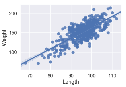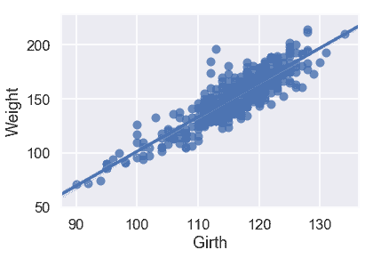 下面是僅使用一個定量變量的三個簡單線性回歸模型。哪一款似乎是最好的？ ``` # HIDDEN sns.regplot('Length', 'Weight', X_train, fit_reg=True); ```  ``` # HIDDEN model = LinearRegression() model.fit(X_train[['Length']], X_train['Weight']) predictions = model.predict(X_test[['Length']]) print("MSE:", mse_test_set(predictions)) ``` ``` MSE: 26052.58007702549 ``` ``` sns.regplot('Girth', 'Weight', X_train, fit_reg=True); ```  ``` # HIDDEN model = LinearRegression() model.fit(X_train[['Girth']], X_train['Weight']) predictions = model.predict(X_test[['Girth']]) print("MSE:", mse_test_set(predictions)) ``` ``` MSE: 13248.814105932383 ``` ``` 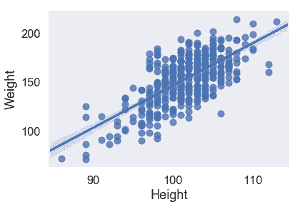sns.regplot('Height', 'Weight', X_train, fit_reg=True); ```  ``` # HIDDEN model = LinearRegression() model.fit(X_train[['Height']], X_train['Weight']) predictions = model.predict(X_test[['Height']]) print("MSE:", mse_test_set(predictions)) ``` ``` MSE: 36343.308584306134 ``` 從散點圖和均方誤差來看，似乎`Girth`是`Weight`的最佳唯一預測因子，因為它與`Weight`具有最強的線性關系，最小的均方誤差。 我們能用兩個變量做得更好嗎？讓我們嘗試使用`Girth`和`Length`來擬合線性模型。雖然這個模型不容易可視化，但是我們仍然可以看到這個模型的 MSE。 ``` # HIDDEN model = LinearRegression() model.fit(X_train[['Girth', 'Length']], X_train['Weight']) predictions = model.predict(X_test[['Girth', 'Length']]) print("MSE:", mse_test_set(predictions)) ``` ``` MSE: 9680.902423377258 ``` 真的！看來我們的 MSE 從 13000 年左右的單用`Girth`下降到 10000 年的單用`Girth`和`Length`。使用包含第二個變量改進了我們的模型。 我們也可以在模型中使用分類變量。現在我們來看一個使用分類變量`Age`的線性模型。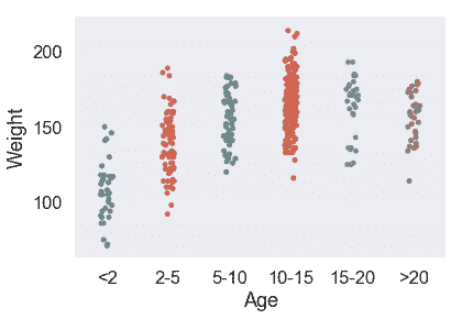這是`Age`與`Weight`的關系圖： ``` # HIDDEN sns.stripplot(x='Age', y='Weight', data=X_train, order=['<2', '2-5', '5-10', '10-15', '15-20', '>20']); ```  考慮到`Age`是一個分類變量，我們需要引入虛擬變量以生成線性回歸模型。 ``` # HIDDEN just_age_and_weight = X_train[['Age', 'Weight']] with_age_dummies = pd.get_dummies(just_age_and_weight, columns=['Age']) model = LinearRegression() model.fit(with_age_dummies.drop('Weight', axis=1), with_age_dummies['Weight']) just_age_and_weight_test = X_test[['Age']] with_age_dummies_test = pd.get_dummies(just_age_and_weight_test, columns=['Age']) predictions = model.predict(with_age_dummies_test) print("MSE:", mse_test_set(predictions)) ``` ``` MSE: 41398.515625 ``` 大約 40000 毫秒比我們使用任何一個定量變量都要差，但是這個變量在我們的線性模型中仍然有用。 讓我們來解釋這個線性模型。請注意，每個屬于年齡類別的驢，例如 2-5 歲，將收到相同的預測，因為它們共享輸入值：1 在列中對應 2-5 歲，0 在所有其他列中。因此，我們可以將分類變量解釋為簡單地改變模型中的常數，因為分類變量將驢分為組，并對該組中的所有驢進行一次預測。 下一步是使用分類變量和多個定量變量創建最終模型。 ## 轉換變量[?](#Transforming-Variables) 回想一下我們的箱線圖`Sex`不是一個有用的變量，所以我們將刪除它。我們還將刪除`WeightAlt`列，因為我們只有 31 頭驢的值。最后，我們使用`get_dummies`將分類變量`BCS`和`Age`轉換為虛擬變量，以便將它們包含在模型中。 ``` # HIDDEN X_train.drop('Weight', axis=1, inplace=True) ``` ``` # HIDDEN pd.set_option('max_columns', 15) ``` ``` X_train.drop(['Sex', 'WeightAlt'], axis=1, inplace=True) X_train = pd.get_dummies(X_train, columns=['BCS', 'Age']) X_train.head() ``` | | Length | Girth | Height | 密件抄送 1.5 | BCS_2.0 | 密件抄送 2.5 | 密件抄送 3.0 | 密件抄送 3.5 | BCS_4.0 | 年齡\10-15 | 年齡 15-20 | 年齡\2-5 | 年齡\5-10 | 年齡 2 | 年齡 20 歲 | | --- | --- | --- | --- | --- | --- | --- | --- | --- | --- | --- | --- | --- | --- | --- | --- | | 四百六十五 | 98 歲 | 一百一十三 | 九十九 | 零 | 0 | 0 | 1 個 | 0 | 0 | 0 | 0 | 1 | 0 | 0 | 0 | | --- | --- | --- | --- | --- | --- | --- | --- | --- | --- | --- | --- | --- | --- | --- | --- | | 233 個 | 101 個 | 一百一十九 | 101 | 0 | 0 | 0 | 1 | 0 | 0 | 1 | 0 | 0 | 0 | 0 | 0 | | --- | --- | --- | --- | --- | --- | --- | --- | --- | --- | --- | --- | --- | --- | --- | --- | | 450 個 | 106 個 | 一百二十五 | 103 個 | 0 | 0 | 1 | 0 | 0 | 0 | 1 | 0 | 0 | 0 | 0 | 0 | | --- | --- | --- | --- | --- | --- | --- | --- | --- | --- | --- | --- | --- | --- | --- | --- | | 四百五十三 | 九十三 | 一百二十 | 100 | 0 | 0 | 1 | 0 | 0 | 0 | 0 | 0 | 1 | 0 | 0 | 0 | | --- | --- | --- | --- | --- | --- | --- | --- | --- | --- | --- | --- | --- | --- | --- | --- | | 452 個 | 98 | 120 | 108 個 | 0 | 0 | 1 | 0 | 0 | 0 | 0 | 0 | 0 | 1 | 0 | 0 | | --- | --- | --- | --- | --- | --- | --- | --- | --- | --- | --- | --- | --- | --- | --- | --- | 回想一下，我們注意到 5 歲以上的驢的體重分布并沒有太大的不同。因此，讓我們將列`Age_10-15`、`Age_15-20`和`Age_&gt;20`組合為一列。 ``` age_over_10 = X_train['Age_10-15'] | X_train['Age_15-20'] | X_train['Age_>20'] X_train['Age_>10'] = age_over_10 X_train.drop(['Age_10-15', 'Age_15-20', 'Age_>20'], axis=1, inplace=True) ``` 因為我們不希望矩陣過度參數化，我們應該從`BCS`和`Age`假人中刪除一個類別。 ``` X_train.drop(['BCS_3.0', 'Age_5-10'], axis=1, inplace=True) X_train.head() ``` | | Length | Girth | Height | BCS_1.5 | BCS_2.0 | BCS_2.5 | BCS_3.5 | BCS_4.0 | Age_2-5 | Age_&lt;2 | 年齡 10 歲 | | --- | --- | --- | --- | --- | --- | --- | --- | --- | --- | --- | --- | | 465 | 98 | 113 | 99 | 0 | 0 | 0 | 0 | 0 | 1 | 0 | 0 | | --- | --- | --- | --- | --- | --- | --- | --- | --- | --- | --- | --- | | 233 | 101 | 119 | 101 | 0 | 0 | 0 | 0 | 0 | 0 | 0 | 1 | | --- | --- | --- | --- | --- | --- | --- | --- | --- | --- | --- | --- | | 450 | 106 | 125 | 103 | 0 | 0 | 1 | 0 | 0 | 0 | 0 | 1 | | --- | --- | --- | --- | --- | --- | --- | --- | --- | --- | --- | --- | | 453 | 93 | 120 | 100 | 0 | 0 | 1 | 0 | 0 | 1 | 0 | 0 | | --- | --- | --- | --- | --- | --- | --- | --- | --- | --- | --- | --- | | 452 | 98 | 120 | 108 | 0 | 0 | 1 | 0 | 0 | 0 | 0 | 0 | | --- | --- | --- | --- | --- | --- | --- | --- | --- | --- | --- | --- | 為了在我們的模型中有一個常數項，我們還應該添加一列偏差。 ``` X_train = X_train.assign(bias=1) ``` ``` # HIDDEN X_train = X_train.reindex(columns=['bias'] + list(X_train.columns[:-1])) ``` ``` X_train.head() ``` | | 偏倚 | Length | Girth | Height | BCS_1.5 | BCS_2.0 | BCS_2.5 | BCS_3.5 | BCS_4.0 | Age_2-5 | Age_&lt;2 | Age_&gt;10 | | --- | --- | --- | --- | --- | --- | --- | --- | --- | --- | --- | --- | --- | | 465 | 1 | 98 | 113 | 99 | 0 | 0 | 0 | 0 | 0 | 1 | 0 | 0 | | --- | --- | --- | --- | --- | --- | --- | --- | --- | --- | --- | --- | --- | | 233 | 1 | 101 | 119 | 101 | 0 | 0 | 0 | 0 | 0 | 0 | 0 | 1 | | --- | --- | --- | --- | --- | --- | --- | --- | --- | --- | --- | --- | --- | | 450 | 1 | 106 | 125 | 103 | 0 | 0 | 1 | 0 | 0 | 0 | 0 | 1 | | --- | --- | --- | --- | --- | --- | --- | --- | --- | --- | --- | --- | --- | | 453 | 1 | 93 | 120 | 100 | 0 | 0 | 1 | 0 | 0 | 1 | 0 | 0 | | --- | --- | --- | --- | --- | --- | --- | --- | --- | --- | --- | --- | --- | | 452 | 1 | 98 | 120 | 108 | 0 | 0 | 1 | 0 | 0 | 0 | 0 | 0 | | --- | --- | --- | --- | --- | --- | --- | --- | --- | --- | --- | --- | --- | ## 多元線性回歸模型 我們終于準備好將我們的模型與我們認為重要的所有變量相匹配，并轉換成適當的形式。 我們的模型如下： $$ f_\theta (\textbf{x}) = \theta_0 + \theta_1 (Length) + \theta_2 (Girth) + \theta_3 (Height) + ... + \theta_{11} (Age_>10) $$ 下面是我們在多元線性回歸課程中定義的函數，我們將再次使用這些函數： ``` def linear_model(thetas, X): '''Returns predictions by a linear model on x_vals.''' return X @ thetas def mse_cost(thetas, X, y): return np.mean((y - linear_model(thetas, X)) ** 2) def grad_mse_cost(thetas, X, y): n = len(X) return -2 / n * (X.T @ y - X.T @ X @ thetas) ``` 為了使用上述函數，我們需要`X`和`y`。這些都可以從我們的數據幀中獲得。記住`X`和`y`必須是 numpy 矩陣，才能用`@`符號將它們相乘。 ``` X_train = X_train.values ``` ``` y_train = y_train.values ``` 現在我們只需要調用在前一節中定義的`minimize`函數。 ``` thetas = minimize(mse_cost, grad_mse_cost, X_train, y_train) ``` ``` theta: [0\. 0\. 0\. 0\. 0\. 0\. 0\. 0\. 0\. 0\. 0\. 0.] | cost: 23979.72 theta: [0.01 0.53 0.65 0.56 0\. 0\. 0\. 0\. 0\. 0\. 0\. 0\. ] | cost: 1214.03 theta: [-0.07 1.84 2.55 -2.87 -0.02 -0.13 -0.34 0.19 0.07 -0.22 -0.3 0.43] | cost: 1002.46 theta: [-0.25 -0.76 4.81 -3.06 -0.08 -0.38 -1.11 0.61 0.24 -0.66 -0.93 1.27] | cost: 815.50 theta: [-0.44 -0.33 4.08 -2.7 -0.14 -0.61 -1.89 1.02 0.4 -1.06 -1.57 2.09] | cost: 491.91 theta: [-1.52 0.85 2\. -1.58 -0.52 -2.22 -5.63 3.29 1.42 -2.59 -5.14 5.54] | cost: 140.86 theta: [-2.25 0.9 1.72 -1.3 -0.82 -3.52 -7.25 4.64 2.16 -2.95 -7.32 6.61] | cost: 130.33 theta: [ -4.16 0.84 1.32 -0.78 -1.65 -7.09 -10.4 7.82 4.18 -3.44 -12.61 8.24] | cost: 116.92 theta: [ -5.89 0.75 1.17 -0.5 -2.45 -10.36 -11.81 10.04 6.08 -3.6 -16.65 8.45] | cost: 110.37 theta: [ -7.75 0.67 1.13 -0.35 -3.38 -13.76 -11.84 11.55 8.2 -3.8 -20\. 7.55] | cost: 105.74 theta: [ -9.41 0.64 1.15 -0.31 -4.26 -16.36 -10.81 11.97 10.12 -4.33 -21.88 6.15] | cost: 102.82 theta: [-11.08 0.66 1.17 -0.32 -5.18 -18.28 -9.43 11.61 11.99 -5.37 -22.77 4.69] | cost: 100.70 theta: [-12.59 0.69 1.16 -0.32 -6.02 -19.17 -8.53 10.86 13.54 -6.65 -22.89 3.73] | cost: 99.34 theta: [-14.2 0.72 1.14 -0.3 -6.89 -19.35 -8.29 10.03 14.98 -7.99 -22.74 3.14] | cost: 98.30 theta: [-16.14 0.73 1.11 -0.26 -7.94 -19.03 -8.65 9.3 16.47 -9.18 -22.59 2.76] | cost: 97.35 theta: [-18.68 0.73 1.1 -0.21 -9.27 -18.29 -9.42 8.76 18.14 -10.04 -22.55 2.39] | cost: 96.38 theta: [-21.93 0.72 1.1 -0.17 -10.94 -17.19 -10.25 8.5 19.92 -10.36 -22.66 1.99] | cost: 95.35 theta: [-26.08 0.7 1.13 -0.14 -13.03 -15.78 -10.79 8.54 21.78 -10.05 -22.83 1.59] | cost: 94.18 theta: [-31.35 0.69 1.17 -0.13 -15.59 -14.12 -10.69 8.9 23.61 -9.19 -22.93 1.32] | cost: 92.84 theta: [-37.51 0.7 1.21 -0.13 -18.44 -12.47 -9.79 9.52 25.14 -8.06 -22.78 1.38] | cost: 91.40 theta: [-43.57 0.72 1.23 -0.12 -21.06 -11.3 -8.4 10.2 25.98 -7.16 -22.24 1.87] | cost: 90.06 theta: [-48.96 0.74 1.23 -0.1 -23.13 -10.82 -7.13 10.76 26.06 -6.79 -21.34 2.6 ] | cost: 88.89 theta: [-54.87 0.76 1.22 -0.05 -25.11 -10.88 -6.25 11.22 25.55 -6.8 -20.04 3.41] | cost: 87.62 theta: [-63.83 0.78 1.21 0.02 -27.82 -11.42 -5.83 11.68 24.36 -6.96 -17.97 4.26] | cost: 85.79 theta: [-77.9 0.8 1.22 0.13 -31.81 -12.47 -6.17 12.03 22.29 -6.98 -14.93 4.9 ] | cost: 83.19 theta: [-94.94 0.81 1.26 0.23 -36.3 -13.73 -7.37 11.98 19.65 -6.47 -11.73 4.88] | cost: 80.40 theta: [-108.1 0.81 1.34 0.28 -39.34 -14.55 -8.72 11.32 17.48 -5.47 -9.92 4.21] | cost: 78.34 theta: [-115.07 0.81 1.4 0.29 -40.38 -14.75 -9.46 10.3 16.16 -4.47 -9.7 3.5 ] | cost: 77.07 theta: [-119.8 0.81 1.44 0.28 -40.43 -14.6 -9.61 9.02 15.09 -3.67 -10.25 3.05] | cost: 76.03 theta: [-125.16 0.82 1.47 0.3 -40.01 -14.23 -9.3 7.48 13.79 -3.14 -11.09 2.94] | cost: 74.96 theta: [-131.24 0.83 1.48 0.33 -39.39 -13.76 -8.71 6.21 12.41 -3.16 -11.79 3.17] | cost: 74.03 theta: [-137.42 0.84 1.48 0.39 -38.62 -13.25 -8.11 5.57 11.18 -3.67 -12.11 3.47] | cost: 73.23 theta: [-144.82 0.85 1.47 0.46 -37.36 -12.53 -7.56 5.47 9.93 -4.57 -12.23 3.56] | cost: 72.28 theta: [-155.48 0.86 1.48 0.54 -34.88 -11.3 -6.98 5.95 8.38 -5.92 -12.27 3.13] | cost: 70.91 theta: [-167.86 0.88 1.52 0.62 -31.01 -9.63 -6.53 7.03 6.9 -7.3 -12.29 1.91] | cost: 69.33 theta: [-176.09 0.89 1.57 0.64 -27.32 -8.32 -6.41 8.07 6.31 -7.84 -12.29 0.44] | cost: 68.19 theta: [-178.63 0.9 1.6 0.62 -25.15 -7.88 -6.5 8.52 6.6 -7.51 -12.19 -0.39] | cost: 67.59 theta: [-179.83 0.91 1.63 0.6 -23.4 -7.84 -6.6 8.61 7.27 -6.83 -11.89 -0.72] | cost: 67.08 theta: [-182.79 0.91 1.66 0.58 -20.55 -8.01 -6.68 8.49 8.44 -5.7 -11.11 -0.69] | cost: 66.27 theta: [-190.23 0.93 1.68 0.6 -15.62 -8.38 -6.68 8.1 10.26 -4.1 -9.46 0.01] | cost: 65.11 theta: [-199.13 0.93 1.69 0.67 -11.37 -8.7 -6.55 7.67 11.53 -3.17 -7.81 1.13] | cost: 64.28 theta: [-203.85 0.93 1.68 0.72 -10.03 -8.78 -6.42 7.5 11.68 -3.25 -7.13 1.86] | cost: 64.01 theta: [-204.24 0.93 1.67 0.74 -10.33 -8.74 -6.39 7.52 11.46 -3.52 -7.17 1.97] | cost: 63.98 theta: [-204.06 0.93 1.67 0.74 -10.48 -8.72 -6.39 7.54 11.39 -3.59 -7.22 1.95] | cost: 63.98 theta: [-204.03 0.93 1.67 0.74 -10.5 -8.72 -6.39 7.54 11.39 -3.6 -7.22 1.95] | cost: 63.98 theta: [-204.03 0.93 1.67 0.74 -10.5 -8.72 -6.39 7.54 11.39 -3.6 -7.22 1.95] | cost: 63.98 theta: [-204.03 0.93 1.67 0.74 -10.5 -8.72 -6.39 7.54 11.39 -3.6 -7.22 1.95] | cost: 63.98 theta: [-204.03 0.93 1.67 0.74 -10.5 -8.72 -6.39 7.54 11.39 -3.6 -7.22 1.95] | cost: 63.98 theta: [-204.03 0.93 1.67 0.74 -10.5 -8.72 -6.39 7.54 11.39 -3.6 -7.22 1.95] | cost: 63.98 theta: [-204.03 0.93 1.67 0.74 -10.5 -8.72 -6.39 7.54 11.39 -3.6 -7.22 1.95] | cost: 63.98 ``` 我們的線性模型是： $Y=-204.03+0.93x_1+…-7.22 倍 9+1.95 倍 11$ 讓我們將我們得到的這個方程與我們使用`sklearn`的線性回歸模型得到的方程進行比較。 ``` model = LinearRegression(fit_intercept=False) # We already accounted for it with the bias column model.fit(X_train[:, :14], y_train) print("Coefficients", model.coef_) ``` ``` Coefficients [-204.03 0.93 1.67 0.74 -10.5 -8.72 -6.39 7.54 11.39 -3.6 -7.22 1.95] ``` 系數看起來完全一樣！我們自制的函數創建了與已建立的 python 包相同的模型！ 我們成功地將線性模型與我們的驢子數據相匹配！尼斯！ ## 評估我們的模型[?](#Evaluating-our-Model) 我們的下一步是在測試集中評估模型的性能。我們需要對測試集執行與培訓集相同的數據預處理步驟，然后才能將其傳遞到我們的模型中。 ``` X_test.drop(['Sex', 'WeightAlt'], axis=1, inplace=True) X_test = pd.get_dummies(X_test, columns=['BCS', 'Age']) age_over_10 = X_test['Age_10-15'] | X_test['Age_15-20'] | X_test['Age_>20'] X_test['Age_>10'] = age_over_10 X_test.drop(['Age_10-15', 'Age_15-20', 'Age_>20'], axis=1, inplace=True) X_test.drop(['BCS_3.0', 'Age_5-10'], axis=1, inplace=True) X_test = X_test.assign(bias=1) ``` ``` # HIDDEN X_test = X_test.reindex(columns=['bias'] + list(X_test.columns[:-1])) ``` ``` X_test ``` | | bias | Length | Girth | Height | BCS_1.5 | BCS_2.0 | BCS_2.5 | BCS_3.5 | BCS_4.0 | Age_2-5 | Age_&lt;2 | Age_&gt;10 | | --- | --- | --- | --- | --- | --- | --- | --- | --- | --- | --- | --- | --- | | 490 個 | 1 | 98 | 119 | 103 | 0 | 0 | 1 | 0 | 0 | 0 | 0 | 1 | | --- | --- | --- | --- | --- | --- | --- | --- | --- | --- | --- | --- | --- | | 75 歲 | 1 | 86 歲 | 一百一十四 | 一百零五 | 0 | 0 | 0 | 0 | 0 | 1 | 0 | 0 | | --- | --- | --- | --- | --- | --- | --- | --- | --- | --- | --- | --- | --- | | 三百五十二 | 1 | 94 | 114 | 101 | 0 | 0 | 0 | 0 | 0 | 0 | 0 | 1 | | --- | --- | --- | --- | --- | --- | --- | --- | --- | --- | --- | --- | --- | | ... | ... | ... | ... | ... | ... | ... | ... | ... | ... | ... | ... | ... | | --- | --- | --- | --- | --- | --- | --- | --- | --- | --- | --- | --- | --- | | 一百八十二 | 1 | 94 | 114 | 一百零二 | 0 | 0 | 0 | 0 | 0 | 1 | 0 | 0 | | --- | --- | --- | --- | --- | --- | --- | --- | --- | --- | --- | --- | --- | | 三百三十四 | 1 | 一百零四 | 113 | 105 | 0 | 0 | 1 | 0 | 0 | 0 | 0 | 0 | | --- | --- | --- | --- | --- | --- | --- | --- | --- | --- | --- | --- | --- | | 五百四十三 | 1 | 104 | 一百二十四 | 一百一十 | 0 | 0 | 0 | 0 | 0 | 0 | 0 | 0 | | --- | --- | --- | --- | --- | --- | --- | --- | --- | --- | --- | --- | --- | 108 行×12 列 我們將`X_test`傳遞到我們的`LinearRegression`模型的`predict`中： ``` X_test = X_test.values predictions = model.predict(X_test) ``` 讓我們看看均方誤差： ``` mse_test_set(predictions) ``` ``` 7261.974205350604 ``` 通過這些預測，我們還可以繪制一個殘差圖： ``` # HIDDEN y_test = y_test.values resid = y_test - predictions resid_prop = resid / y_test plt.scatter(np.arange(len(resid_prop)), resid_prop, s=15) plt.axhline(0) plt.title('Residual proportions (resid / actual Weight)') plt.xlabel('Index of row in data') plt.ylabel('Error proportion'); ```  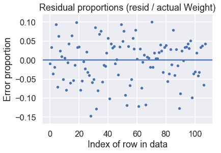看起來我們的模型做得很好！剩余比例表明，我們的預測大多在正確值的 15%以內。