# 多元線性回歸 > 原文：[https://www.bookbookmark.ds100.org/ch/13/linear_multiple.html](https://www.bookbookmark.ds100.org/ch/13/linear_multiple.html) ``` # HIDDEN # Clear previously defined variables %reset -f # Set directory for data loading to work properly import os os.chdir(os.path.expanduser('~/notebooks/13')) ``` ``` # HIDDEN import warnings # Ignore numpy dtype warnings. These warnings are caused by an interaction # between numpy and Cython and can be safely ignored. # Reference: https://stackoverflow.com/a/40846742 warnings.filterwarnings("ignore", message="numpy.dtype size changed") warnings.filterwarnings("ignore", message="numpy.ufunc size changed") import numpy as np import matplotlib.pyplot as plt import pandas as pd import seaborn as sns %matplotlib inline import ipywidgets as widgets from ipywidgets import interact, interactive, fixed, interact_manual import nbinteract as nbi sns.set() sns.set_context('talk') np.set_printoptions(threshold=20, precision=2, suppress=True) pd.options.display.max_rows = 7 pd.options.display.max_columns = 8 pd.set_option('precision', 2) # This option stops scientific notation for pandas # pd.set_option('display.float_format', '{:.2f}'.format) ``` ``` # HIDDEN def df_interact(df, nrows=7, ncols=7): ''' Outputs sliders that show rows and columns of df ''' def peek(row=0, col=0): return df.iloc[row:row + nrows, col:col + ncols] if len(df.columns) <= ncols: interact(peek, row=(0, len(df) - nrows, nrows), col=fixed(0)) else: interact(peek, row=(0, len(df) - nrows, nrows), col=(0, len(df.columns) - ncols)) print('({} rows, {} columns) total'.format(df.shape[0], df.shape[1])) ``` ``` # HIDDEN from scipy.optimize import minimize as sci_min def minimize(loss_fn, grad_loss_fn, X, y, progress=True): ''' Uses scipy.minimize to minimize loss_fn using a form of gradient descent. ''' theta = np.zeros(X.shape[1]) iters = 0 def objective(theta): return loss_fn(theta, X, y) def gradient(theta): return grad_loss_fn(theta, X, y) def print_theta(theta): nonlocal iters if progress and iters % progress == 0: print(f'theta: {theta} | loss: {loss_fn(theta, X, y):.2f}') iters += 1 print_theta(theta) return sci_min( objective, theta, method='BFGS', jac=gradient, callback=print_theta, tol=1e-7 ).x ``` 與常量模型相比，我們的簡單線性模型有一個關鍵優勢：它在進行預測時使用數據。然而，由于簡單的線性模型在我們的數據集中只使用一個變量，所以它仍然相當有限。許多數據集都有許多潛在的有用變量，多元線性回歸可以利用這一點。例如，考慮以下有關車型及其每加侖里程（mpg）的數據集： ``` mpg = pd.read_csv('mpg.csv').dropna().reset_index(drop=True) mpg ``` | | MPG | 氣缸 | 取代 | …… | 車型年份 | 起源 | 車名 | | --- | --- | --- | --- | --- | --- | --- | --- | | 零 | 18.0 條 | 8 個 | 三百零七 | …… | 70 個 | 1 個 | 雪佛蘭 Chevelle Malibu | | --- | --- | --- | --- | --- | --- | --- | --- | | 1 個 | 15.0 條 | 8 | 三百五十 | ... | 70 | 1 | 別克云雀 320 | | --- | --- | --- | --- | --- | --- | --- | --- | | 二 | 18.0 | 8 | 三百一十八 | ... | 70 | 1 | 普利茅斯衛星 | | --- | --- | --- | --- | --- | --- | --- | --- | | ... | ... | ... | ... | ... | ... | ... | ... | | --- | --- | --- | --- | --- | --- | --- | --- | | 三百八十九 | 32.0 美元 | 四 | 一百三十五 | ... | 八十二 | 1 | 躲避暴行 | | --- | --- | --- | --- | --- | --- | --- | --- | | 三百九十 | 二十八 | 4 | 一百二十 | ... | 82 | 1 | 福特漫游者 | | --- | --- | --- | --- | --- | --- | --- | --- | | 391 個 | 三十一 | 4 | 一百一十九 | ... 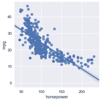| 82 | 1 | 雪佛蘭 S-10 | | --- | --- | --- | --- | --- | --- | --- | --- | 392 行×9 列 汽車模型的多個屬性似乎會影響其 MPG。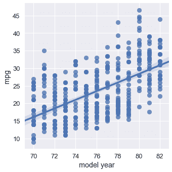例如，MPG 似乎隨著馬力的增加而降低： ``` # HIDDEN sns.lmplot(x='horsepower', y='mpg', data=mpg); ```  然而，稍后發布的汽車通常比舊款汽車具有更好的 MPG： ``` sns.lmplot(x='model year', y='mpg', data=mpg); ```  如果我們能在預測 MPG 時同時考慮馬力和車型年份，我們就有可能得到更精確的模型。事實上，最好的模型可能會考慮到數據集中的所有數值變量。我們可以擴展單變量線性回歸，以允許基于任意數量的屬性進行預測。 我們陳述了以下模型： $$ f_\boldsymbol\theta (\textbf{x}) = \theta_0 + \theta_1 x_1 + \ldots + \theta_p x_p $$ 其中，$\textbf x$現在表示包含單個汽車$p$屬性的向量。上面的模型說，“取一輛車的多個屬性，乘以一些權重，然后將它們相加，對 MPG 做出預測。” 例如，如果我們使用“馬力”、“重量”和“車型年”列對數據集中的第一輛車進行預測，那么向量$\textbf x$ ``` # HIDDEN mpg.loc[0:0, ['horsepower', 'weight', 'model year']] ``` | | 馬力 | 重量 | model year | | --- | --- | --- | --- | | 0 | 一百三十 | 三千五百零四 | 70 | | --- | --- | --- | --- | 在這里的例子中，為了清晰起見，我們保留了列名，但要記住，$\textbf x$只包含上表的數值：$\textbf x=[130.0，3504.0，70]$。 現在，我們將執行一個符號技巧，它將大大簡化后面的公式。我們將在向量$\textbf x 中預先設置$1$的值，這樣我們就可以為$\textbf x 獲得以下向量： ``` # HIDDEN mpg_mat = mpg.assign(bias=1) mpg_mat.loc[0:0, ['bias', 'horsepower', 'weight', 'model year']] ``` | | 偏倚 | horsepower | weight | model year | | --- | --- | --- | --- | --- | | 0 | 1 | 130.0 | 3504.0 | 70 | | --- | --- | --- | --- | --- | 現在，觀察我們模型的公式發生了什么： $$ \begin{aligned} f_\boldsymbol\theta (\textbf{x}) &= \theta_0 + \theta_1 x_1 + \ldots + \theta_p x_p \\ &= \theta_0 (1) + \theta_1 x_1 + \ldots + \theta_p x_p \\ &= \theta_0 x_0 + \theta_1 x_1 + \ldots + \theta_p x_p \\ f_\boldsymbol\theta (\textbf{x}) &= \boldsymbol\theta \cdot \textbf{x} \end{aligned} $$ 其中，$\boldSymbol\theta\cdot\textbf x$是$\boldSymbol\theta$和$\textbf x$的矢量點積。矢量和矩陣表示法被設計成簡潔地寫線性組合，因此非常適合我們的線性模型。但是，從現在開始你必須記住，$\BoldSymbol\Theta\CDOT\textBF x$是矢量點積。如果有疑問，可以將點積展開為簡單的乘法和加法。 現在，我們將矩陣$\textbf x 定義為包含每個車型的矩陣，作為一行和第一列偏差。例如，下面是前五行$\textbf x$： ``` # HIDDEN mpg_mat = mpg.assign(bias=1) mpg_mat.loc[0:4, ['bias', 'horsepower', 'weight', 'model year']] ``` | | bias | horsepower | weight | model year | | --- | --- | --- | --- | --- | | 0 | 1 | 130.0 | 3504.0 | 70 | | --- | --- | --- | --- | --- | | 1 | 1 | 一百六十五 | 三千六百九十三 | 70 | | --- | --- | --- | --- | --- | | 2 | 1 | 一百五十 | 三千四百三十六 | 70 | | --- | --- | --- | --- | --- | | 三 | 1 | 150.0 | 三千四百三十三 | 70 | | --- | --- | --- | --- | --- | | 四 | 1 | 一百四十 | 三千四百四十九 | 70 | | --- | --- | --- | --- | --- | 同樣，請記住，實際矩陣$\textbf x$只包含上表的數值。 注意，$\textbf x$由多個疊加在一起的$\textbf x$向量組成。為了保持符號清晰，我們定義了$\textbf x i$以引用索引為$i$的行向量，索引為$i$of$\textbf x$。我們定義$x_i，j$以引用索引為$j$的元素，索引為$i$的行的索引為$textbf x$。因此，$\textbf x u i$是一個$p$維向量，$x i，j$是一個標量。$\textbf x$是一個$n \乘以 p$矩陣，其中$n$是我們擁有的汽車示例數量，$p$是我們擁有的單個汽車的屬性數量。 例如，從上表中，我們有$\textbf x u 4=[1，140，3449，70]$和$x 4，1=140$。當我們定義損失函數時，這個符號變得很重要，因為我們需要輸入值的矩陣$\textbf x$，以及 MPG 的向量$\textbf y$。 ## MSE 損耗及其梯度 均方誤差損失函數采用一個權重為$\BoldSymbol\Theta$的向量、一個輸入矩陣$\textbf x 和一個觀察到的 mpgs 的向量$\textbf y： $$ \begin{aligned} L(\boldsymbol\theta, \textbf{X}, \textbf{y}) &= \frac{1}{n} \sum_{i}(y_i - f_\boldsymbol\theta (\textbf{X}_i))^2\\ \end{aligned} $$ 我們之前已經推導了 mse 損失相對于$\BoldSymbol\Theta$的梯度： $$ \begin{aligned} \nabla_{\boldsymbol\theta} L(\boldsymbol\theta, \textbf{X}, \textbf{y}) &= -\frac{2}{n} \sum_{i}(y_i - f_\boldsymbol\theta (\textbf{X}_i))(\nabla_{\boldsymbol\theta} f_\boldsymbol\theta (\textbf{X}_i))\\ \end{aligned} $$ 我們知道： $$ \begin{aligned} f_\boldsymbol\theta (\textbf{x}) &= \boldsymbol\theta \cdot \textbf{x} \\ \end{aligned} $$ 現在讓我們計算$\nabla_ \boldsymbol\theta_f_boldsymbol\theta（\textbf_x）$。結果是非常簡單的，因為$\boldsymbol\theta\cdot\textbf x；=\theta x _0+\ldots+\theta p x _p$和因此\frac \ \部分 \ \部分\theta（\boldsy \\theta\cdot\textbf x）=x 美元，$\frac \ \ \ \部分部分\ \\theta（（\boldsy 符號 theta\cdot\textbf x）=x_1$等在。 $$ \begin{aligned} \nabla_{\boldsymbol\theta} f_\boldsymbol\theta (\textbf{x}) &= \nabla_{\boldsymbol\theta} [ \boldsymbol\theta \cdot \textbf{x} ] \\ &= \begin{bmatrix} \frac{\partial}{\partial \theta_0} (\boldsymbol\theta \cdot \textbf{x}) \\ \frac{\partial}{\partial \theta_1} (\boldsymbol\theta \cdot \textbf{x}) \\ \vdots \\ \frac{\partial}{\partial \theta_p} (\boldsymbol\theta \cdot \textbf{x}) \\ \end{bmatrix} \\ &= \begin{bmatrix} x_0 \\ x_1 \\ \vdots \\ x_p \end{bmatrix} \\ \nabla_{\boldsymbol\theta} f_\boldsymbol\theta (\textbf{x}) &= \textbf{x} \end{aligned} $$ 最后，我們將此結果插入到我們的梯度計算中： $$ \begin{aligned} \nabla_{\boldsymbol\theta} L(\boldsymbol\theta, \textbf{X}, \textbf{y}) &= -\frac{2}{n} \sum_{i}(y_i - f_\boldsymbol\theta (\textbf{X}_i))(\nabla_{\boldsymbol\theta} f_\boldsymbol\theta (\textbf{X}_i))\\ &= -\frac{2}{n} \sum_{i}(y_i - \boldsymbol\theta \cdot \textbf{X}_i)(\textbf{X}_i)\\ \end{aligned} $$ 請記住，既然$y_i-\boldsymbol\theta\cdot\textbf x u i$是一個標量，而$textbf x u i$是一個$p$維向量，那么梯度$nabla \boldsymbol\theta l（\boldsymbol\theta、\textbf x、\textbf y）是一個$p$維向量。 當我們計算單變量線性回歸的梯度時，我們看到了相同類型的結果，發現它是二維的，因為$\BoldSymbol\Theta$是二維的。 ## 用梯度下降法擬合模型 我們現在可以把損失及其導數代入梯度下降。和往常一樣，我們將在 python 中定義模型、損失和漸變損失。 ``` def linear_model(thetas, X): '''Returns predictions by a linear model on x_vals.''' return \textbf{X} @ thetas def mse_loss(thetas, X, y): return np.mean((y - linear_model(thetas, X)) ** 2) def grad_mse_loss(thetas, X, y): n = len(X) return -2 / n * (X.T @ \textbf{y} - X.T @ \textbf{X} @ thetas) ``` ``` # HIDDEN thetas = np.array([1, 1, 1, 1]) \textbf{X} = np.array([[2, 1, 0, 1], [1, 2, 3, 4]]) y = np.array([3, 9]) assert np.allclose(linear_model(thetas, X), [4, 10]) assert np.allclose(mse_loss(thetas, X, y), 1.0) assert np.allclose(grad_mse_loss(thetas, X, y), [ 3., 3., 3., 5.]) assert np.allclose(grad_mse_loss(thetas, \textbf{X} + 1, y), [ 25., 25., 25., 35.]) ``` 現在，我們可以簡單地將函數插入梯度下降最小化器： ``` # HIDDEN \textbf{X} = (mpg_mat .loc[:, ['bias', 'horsepower', 'weight', 'model year']] .as_matrix()) y = mpg_mat['mpg'].as_matrix() ``` ``` %%time thetas = minimize(mse_loss, grad_mse_loss, X, y) print(f'theta: {thetas} | loss: {mse_loss(thetas, X, y):.2f}') ``` ``` theta: [ 0\. 0\. 0\. 0.] | cost: 610.47 theta: [ 0\. 0\. 0.01 0\. ] | cost: 178.95 theta: [ 0.01 -0.11 -0\. 0.55] | cost: 15.78 theta: [ 0.01 -0.01 -0.01 0.58] | cost: 11.97 theta: [-4\. -0.01 -0.01 0.63] | cost: 11.81 theta: [-13.72 -0\. -0.01 0.75] | cost: 11.65 theta: [-13.72 -0\. -0.01 0.75] | cost: 11.65 CPU times: user 8.81 ms, sys: 3.11 ms, total: 11.9 ms Wall time: 9.22 ms ``` 根據梯度下降，我們的線性模型是： $Y=-13.72-0.01x_2+0.75x_3$ ## 可視化我們的預測 我們的模型怎么樣？我們可以看到損失大幅下降（從 610 下降到 11.6）。我們可以顯示模型的預測值以及原始值： ``` # HIDDEN reordered = ['predicted_mpg', 'mpg', 'horsepower', 'weight', 'model year'] with_predictions = ( mpg .assign(predicted_mpg=linear_model(thetas, X)) .loc[:, reordered] ) with_predictions ``` | | 預測值 | mpg | horsepower | weight | model year | | --- | --- | --- | --- | --- | --- | | 0 | 15.447125 | 18.0 | 130.0 | 3504.0 | 70 | | --- | --- | --- | --- | --- | --- | | 1 | 14.053509 年 | 15.0 | 165.0 | 3693.0 | 70 | | --- | --- | --- | --- | --- | --- | | 2 | 15.785576 個 | 18.0 | 150.0 | 3436.0 | 70 | | --- | --- | --- | --- | --- | --- | | ... | ... | ... | ... | ... | ... | | --- | --- | --- | --- | --- | --- | | 389 | 32.456900 | 32.0 | 八十四 | 二千二百九十五 | 82 | | --- | --- | --- | --- | --- | --- | | 390 | 30.354143 號 | 28.0 | 79.0 美元 | 二千六百二十五 | 82 | | --- | --- | --- | --- | --- | --- | | 391 | 29.726608 | 31.0 | 八十二 | 二千七百二十 | 82 | | --- | --- | --- | --- | --- | --- | 392 行×5 列 由于我們從梯度下降中找到了$\BoldSymbol\Theta$數據，因此我們可以驗證第一行數據的$\BoldSymbol\Theta\CDOT\textbf x u 0$與我們上面的預測相匹配： ``` print(f'Prediction for first row: ' f'{thetas[0] + thetas[1] * 130 + thetas[2] * 3504 + thetas[3] * 70:.2f}') ``` ``` Prediction for first row: 15.45 ``` 我們在下面包含了一個小部件來瀏覽預測和用于進行預測的數據： ``` # HIDDEN df_interact(with_predictions) ``` <button class="js-nbinteract-widget">Loading widgets...</button> ``` (392 rows, 5 columns) total ``` 我們還可以繪制預測的殘差（實際值-預測值）： ``` resid = \textbf{y} - linear_model(thetas, X) plt.scatter(np.arange(len(resid)), resid, s=15) plt.title('Residuals (actual MPG - predicted MPG)') plt.xlabel('Index of row in data') plt.ylabel('MPG'); ```  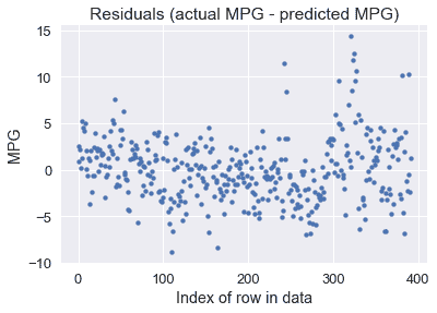看起來我們的模型對許多車型做出了合理的預測，盡管有一些預測超過了每加侖 10 英里（有些車型低于每加侖 10 英里）。。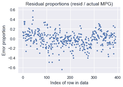也許我們對預測的 MPG 值和實際的 MPG 值之間的百分比誤差更感興趣： ``` resid_prop = resid / with_predictions['mpg'] plt.scatter(np.arange(len(resid_prop)), resid_prop, s=15) plt.title('Residual proportions (resid / actual MPG)') plt.xlabel('Index of row in data') plt.ylabel('Error proportion'); ```  看起來我們模型的預測值通常與實際 MPG 值相差 20%以內。 ## 使用所有數據[?](#Using-All-the-Data) 請注意，到目前為止，我們的示例中，$\textbf x$矩陣有四列：一列是所有列中的一列，馬力、重量和車型年份。但是，模型允許我們處理任意數量的列： $$ \begin{aligned} f_\boldsymbol\theta (\textbf{x}) &= \boldsymbol\theta \cdot \textbf{x} \end{aligned} $$ 當我們在數據矩陣中包含更多的列時，我們擴展了$\BoldSymbol\Theta$以便它在$\textbf x$中為每一列都有一個參數。與其只選擇三個數值列進行預測，為什么不全部使用這七個數值列呢？ ``` # HIDDEN cols = ['bias', 'cylinders', 'displacement', 'horsepower', 'weight', 'acceleration', 'model year', 'origin'] \textbf{X} = mpg_mat[cols].as_matrix() mpg_mat[cols] ``` | | bias | cylinders | displacement | ... | 加快 | model year | origin | | --- | --- | --- | --- | --- | --- | --- | --- | | 0 | 1 | 8 | 307.0 | ... | 十二 | 70 | 1 | | --- | --- | --- | --- | --- | --- | --- | --- | | 1 | 1 | 8 | 350.0 | ... | 十一點五 | 70 | 1 | | --- | --- | --- | --- | --- | --- | --- | --- | | 2 | 1 | 8 | 318.0 | ... | 11.0 條 | 70 | 1 | | --- | --- | --- | --- | --- | --- | --- | --- | | ... | ... | ... | ... | ... | ... | ... | ... | | --- | --- | --- | --- | --- | --- | --- | --- | | 389 | 1 | 4 | 135.0 | ... | 十一點六 | 82 | 1 | | --- | --- | --- | --- | --- | --- | --- | --- | | 390 | 1 | 4 | 120.0 | ... | 十八點六 | 82 | 1 | | --- | --- | --- | --- | --- | --- | --- | --- | | 391 | 1 | 4 | 119.0 | ... | 十九點四 | 82 | 1 | | --- | --- | --- | --- | --- | --- | --- | --- | 392 行×8 列 ``` %%time thetas_all = minimize(mse_loss, grad_mse_loss, X, y, progress=10) print(f'theta: {thetas_all} | loss: {mse_loss(thetas_all, X, y):.2f}') ``` ``` theta: [ 0\. 0\. 0\. 0\. 0\. 0\. 0\. 0.] | cost: 610.47 theta: [-0.5 -0.81 0.02 -0.04 -0.01 -0.07 0.59 1.3 ] | cost: 11.22 theta: [-17.23 -0.49 0.02 -0.02 -0.01 0.08 0.75 1.43] | cost: 10.85 theta: [-17.22 -0.49 0.02 -0.02 -0.01 0.08 0.75 1.43] | cost: 10.85 CPU times: user 10.9 ms, sys: 3.51 ms, total: 14.4 ms Wall time: 11.7 ms ``` According to gradient descent, our linear model is: $Y=-17.22-0.49x_1+0.02x_2-0.02x_3-0.01x_4+0.08X_5+0.75x_6+1.43x_7$ 我們發現，當使用數據集的所有七個數值列時，我們的損失已經從數據集的三列 11.6 減少到了 10.85。我們在下面顯示舊預測和新預測的比例誤差圖： ``` # HIDDEN resid_prop_all = (y - linear_model(thetas_all, X)) / with_predictions['mpg'] plt.figure(figsize=(10, 4)) plt.subplot(121) plt.scatter(np.arange(len(resid_prop)), resid_prop, s=15) plt.title('Residual proportions using 3 columns') plt.xlabel('Index of row in data') plt.ylabel('Error proportion') plt.ylim(-0.7, 0.7) plt.subplot(122) plt.scatter(np.arange(len(resid_prop_all)), resid_prop_all, s=15) plt.title('Residual proportions using 7 columns') plt.xlabel('Index of row in data') plt.ylabel('Error proportion') plt.ylim(-0.7, 0.7) plt.tight_layout(); ```  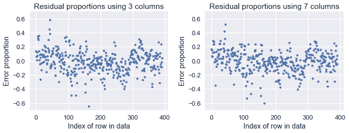雖然差異很小，但與使用三列相比，使用七列時的錯誤要低一些。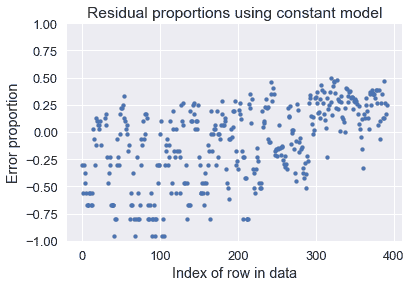兩種模型都比使用常量模型要好得多，如下圖所示： ``` # HIDDEN constant_resid_prop = (y - with_predictions['mpg'].mean()) / with_predictions['mpg'] plt.scatter(np.arange(len(constant_resid_prop)), constant_resid_prop, s=15) plt.title('Residual proportions using constant model') plt.xlabel('Index of row in data') plt.ylabel('Error proportion') plt.ylim(-1, 1); ```  使用一個恒定的模型會導致許多汽車 MPG 超過 75%的誤差！ ## 摘要[?](#Summary) 我們引入了回歸的線性模型。與常數模型不同，線性回歸模型在進行預測時考慮了數據的特征，這使得當我們的數據變量之間存在相關性時，線性回歸模型更加有用。 模型與數據的擬合過程現在應該非常熟悉了： 1. 選擇一個模型。 2. 選擇損失函數。 3. 使用梯度下降最小化損失函數。 知道我們通常可以在不更改其他組件的情況下調整其中一個組件是很有用的。在這一部分中，我們引入了線性模型，沒有改變我們的損失函數或使用不同的最小化算法。雖然建模會變得復雜，但通常通過一次只關注一個組件，然后根據實際需要將不同的部分組合在一起，更容易學習。