# 用梯度下降擬合線性模型 > 原文：[https://www.textbook.ds100.org/ch/13/linear_grad.html](https://www.textbook.ds100.org/ch/13/linear_grad.html) ``` # HIDDEN # Clear previously defined variables %reset -f # Set directory for data loading to work properly import os os.chdir(os.path.expanduser('~/notebooks/13')) ``` ``` # HIDDEN import warnings # Ignore numpy dtype warnings. These warnings are caused by an interaction # between numpy and Cython and can be safely ignored. # Reference: https://stackoverflow.com/a/40846742 warnings.filterwarnings("ignore", message="numpy.dtype size changed") warnings.filterwarnings("ignore", message="numpy.ufunc size changed") import numpy as np import matplotlib.pyplot as plt import pandas as pd import seaborn as sns %matplotlib inline import ipywidgets as widgets from ipywidgets import interact, interactive, fixed, interact_manual import nbinteract as nbi sns.set() sns.set_context('talk') np.set_printoptions(threshold=20, precision=2, suppress=True) pd.options.display.max_rows = 7 pd.options.display.max_columns = 8 pd.set_option('precision', 2) # This option stops scientific notation for pandas # pd.set_option('display.float_format', '{:.2f}'.format) ``` ``` # HIDDEN tips = sns.load_dataset('tips') ``` ``` # HIDDEN def minimize(loss_fn, grad_loss_fn, x_vals, y_vals, alpha=0.0005, progress=True): ''' Uses gradient descent to minimize loss_fn. Returns the minimizing value of theta once the loss changes less than 0.0001 between iterations. ''' theta = np.array([0., 0.]) loss = loss_fn(theta, x_vals, y_vals) while True: if progress: print(f'theta: {theta} | loss: {loss}') gradient = grad_loss_fn(theta, x_vals, y_vals) new_theta = theta - alpha * gradient new_loss = loss_fn(new_theta, x_vals, y_vals) if abs(new_loss - loss) < 0.0001: return new_theta theta = new_theta loss = new_loss ``` 我們希望擬合一個線性模型，該模型根據表中的總賬單預測小費金額： $$ f_\boldsymbol\theta (x) = \theta_1 x + \theta_0 $$ 為了優化$\Theta_1$和$\Theta_0$，我們需要首先選擇一個損失函數。我們將選擇均方誤差損失函數： $$ \begin{aligned} L(\boldsymbol\theta, \textbf{x}, \textbf{y}) &= \frac{1}{n} \sum_{i = 1}^{n}(y_i - f_\boldsymbol\theta (x_i))^2\\ \end{aligned} $$ 請注意，我們已經修改了損失函數，以反映在新模型中添加的解釋變量。現在，$\textbf x$是一個包含單個總賬單的向量，$\textbf y$是一個包含單個小費金額的向量，$\boldsymbol\theta$是一個向量：$\boldsymbol\theta=[\theta\u 1，\theta\u 0]$。 使用帶平方誤差的線性模型也可以用最小二乘線性回歸的名稱。我們可以使用漸變下降來找到能將損失最小化的$\BoldSymbol\Theta$。 **關于使用相關性的旁白** 如果您以前見過最小二乘線性回歸，您可能會認識到我們可以計算相關系數，并用它來確定$\theta_1$和$\theta_0$。對于這個特定的問題，這比使用梯度下降法計算更簡單、更快，類似于計算平均值比使用梯度下降法擬合常量模型更簡單。不管怎樣，我們都會使用梯度下降，因為它是一種通用的損失最小化方法，當我們稍后引入沒有解析解的模型時仍然有效。事實上，在許多現實場景中，即使存在分析解，我們也會使用梯度下降，因為計算分析解比梯度下降要花更長的時間，尤其是在大型數據集上。 ## MSE 損失的導數[?](#Derivative-of-the-MSE-Loss) 為了使用梯度下降，我們必須計算 MSE 損失相對于$\BoldSymbol\Theta$的導數。既然$\BoldSymbol\Theta$是長度為 2 的向量，而不是標量，$\nabla \BoldSymbol\Theta l（\BoldSymbol\Theta、\textbf x、\textbf y）$也將是長度為 2 的向量。 $$ \begin{aligned} \nabla_{\boldsymbol\theta} L(\boldsymbol\theta, \textbf{x}, \textbf{y}) &= \nabla_{\boldsymbol\theta} \left[ \frac{1}{n} \sum_{i = 1}^{n}(y_i - f_\boldsymbol\theta (x_i))^2 \right] \\ &= \frac{1}{n} \sum_{i = 1}^{n}2 (y_i - f_\boldsymbol\theta (x_i))(- \nabla_{\boldsymbol\theta} f_\boldsymbol\theta (x_i))\\ &= -\frac{2}{n} \sum_{i = 1}^{n}(y_i - f_\boldsymbol\theta (x_i))(\nabla_{\boldsymbol\theta} f_\boldsymbol\theta (x_i))\\ \end{aligned} $$ 我們知道： $$ f_\boldsymbol\theta (x) = \theta_1 x + \theta_0 $$ 我們現在需要計算$\nabla_ \boldsymbol\theta_f UuBoldsymbol\theta（x_i）$這是一個長度為 2 的向量。 $$ \begin{aligned} \nabla_{\boldsymbol\theta} f_\boldsymbol\theta (x_i) &= \begin{bmatrix} \frac{\partial}{\partial \theta_0} f_\boldsymbol\theta (x_i)\\ \frac{\partial}{\partial \theta_1} f_\boldsymbol\theta (x_i) \end{bmatrix} \\ &= \begin{bmatrix} \frac{\partial}{\partial \theta_0} [\theta_1 x_i + \theta_0]\\ \frac{\partial}{\partial \theta_1} [\theta_1 x_i + \theta_0] \end{bmatrix} \\ &= \begin{bmatrix} 1 \\ x_i \end{bmatrix} \\ \end{aligned} $$ 最后，我們再回到上面的公式中，得到 $$ \begin{aligned} \nabla_{\boldsymbol\theta} L(\theta, \textbf{x}, \textbf{y}) &= -\frac{2}{n} \sum_{i = 1}^{n}(y_i - f_\boldsymbol\theta (x_i))(\nabla_{\boldsymbol\theta} f_\boldsymbol\theta (x_i))\\ &= -\frac{2}{n} \sum_{i = 1}^{n} (y_i - f_\boldsymbol\theta (x_i)) \begin{bmatrix} 1 \\ x_i \end{bmatrix} \\ &= -\frac{2}{n} \sum_{i = 1}^{n} \begin{bmatrix} (y_i - f_\boldsymbol\theta (x_i)) \\ (y_i - f_\boldsymbol\theta (x_i)) x_i \end{bmatrix} \\ \end{aligned} $$ 這是一個長度為 2 的向量，因為$（y_i-f_uuBoldSymbol\theta（x_i））$是標量。 ## 運行梯度下降 現在，讓我們在 tip s 數據集上擬合一個線性模型，從總表賬單中預測 tip 金額。 首先，我們定義一個 python 函數來計算損失： ``` def simple_linear_model(thetas, x_vals): '''Returns predictions by a linear model on x_vals.''' return thetas[0] + thetas[1] * x_vals def mse_loss(thetas, x_vals, y_vals): return np.mean((y_vals - simple_linear_model(thetas, x_vals)) ** 2) ``` 然后，我們定義一個函數來計算損失的梯度： ``` def grad_mse_loss(thetas, x_vals, y_vals): n = len(x_vals) grad_0 = y_vals - simple_linear_model(thetas, x_vals) grad_1 = (y_vals - simple_linear_model(thetas, x_vals)) * x_vals return -2 / n * np.array([np.sum(grad_0), np.sum(grad_1)]) ``` ``` # HIDDEN thetas = np.array([1, 1]) x_vals = np.array([3, 4]) y_vals = np.array([4, 5]) assert np.allclose(grad_mse_loss(thetas, x_vals, y_vals), [0, 0]) ``` 我們將使用前面定義的`minimize`函數，它運行梯度下降，解釋新的解釋變量。它具有函數簽名（省略正文）： ``` minimize(loss_fn, grad_loss_fn, x_vals, y_vals) ``` 最后，我們進行梯度下降！ ``` %%time thetas = minimize(mse_loss, grad_mse_loss, tips['total_bill'], tips['tip']) ``` ``` theta: [0\. 0.] | cost: 10.896283606557377 theta: [0\. 0.07] | cost: 3.8937622006094705 theta: [0\. 0.1] | cost: 1.9359443267168215 theta: [0.01 0.12] | cost: 1.388538448286097 theta: [0.01 0.13] | cost: 1.235459416905535 theta: [0.01 0.14] | cost: 1.1926273731479433 theta: [0.01 0.14] | cost: 1.1806184944517062 theta: [0.01 0.14] | cost: 1.177227251696266 theta: [0.01 0.14] | cost: 1.1762453624313751 theta: [0.01 0.14] | cost: 1.1759370980989148 theta: [0.01 0.14] | cost: 1.175817178966766 CPU times: user 272 ms, sys: 67.3 ms, total: 339 ms Wall time: 792 ms ``` 我們可以看到梯度下降收斂到θ的值，即，θ0=0.01 美元，θ1=0.14 美元。我們的線性模型是： $$y = 0.14x + 0.01$$ 我們可以使用我們的估計θ，在原始數據點的旁邊做出和繪制預測。 ``` # HIDDEN x_vals = np.array([0, 55]) sns.lmplot(x='total_bill', y='tip', data=tips, fit_reg=False) plt.plot(x_vals, simple_linear_model(thetas, x_vals), c='goldenrod') plt.title('Tip amount vs. 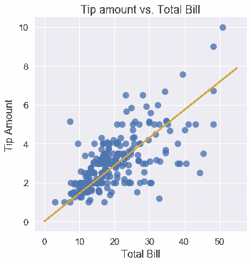Total Bill') plt.xlabel('Total Bill') plt.ylabel('Tip Amount'); ```  我們可以看到，如果一張桌子的帳單是 10 美元，我們的模型將預測服務員得到大約 1.50 美元的小費。同樣，如果一張表的帳單是 40 美元，我們的模型將預測大約 6 美元的小費。