# 多類分類 > 原文：[https://www.textbook.ds100.org/ch/17/classification_multicolass.html](https://www.textbook.ds100.org/ch/17/classification_multicolass.html) ``` # HIDDEN # Clear previously defined variables %reset -f # Set directory for data loading to work properly import os os.chdir(os.path.expanduser('~/notebooks/17')) ``` ``` # HIDDEN import warnings # Ignore numpy dtype warnings. These warnings are caused by an interaction # between numpy and Cython and can be safely ignored. # Reference: https://stackoverflow.com/a/40846742 warnings.filterwarnings("ignore", message="numpy.dtype size changed") warnings.filterwarnings("ignore", message="numpy.ufunc size changed") import numpy as np import matplotlib.pyplot as plt import pandas as pd import seaborn as sns %matplotlib inline import ipywidgets as widgets from ipywidgets import interact, interactive, fixed, interact_manual import nbinteract as nbi sns.set() sns.set_context('talk') np.set_printoptions(threshold=20, precision=2, suppress=True) pd.options.display.max_rows = 7 pd.options.display.max_columns = 8 pd.set_option('precision', 2) # This option stops scientific notation for pandas # pd.set_option('display.float_format', '{:.2f}'.format) ``` ``` # HIDDEN markers = {'triangle':['^', sns.color_palette()[0]], 'square':['s', sns.color_palette()[1]], 'circle':['o', sns.color_palette()[2]]} def plot_binary(data, label): data_copy = data.copy() data_copy['$y$ == ' + label] = (data_copy['$y$'] == label).astype('category') sns.lmplot('$x_1$', '$x_2$', data=data_copy, hue='$y$ == ' + label, hue_order=[True, False], markers=[markers[label][0], 'x'], palette=[markers[label][1], 'gray'], fit_reg=False) plt.xlim(1.0, 4.0) plt.ylim(1.0, 4.0); ``` ``` # HIDDEN def plot_confusion_matrix(y_test, y_pred): sns.heatmap(confusion_matrix(y_test, y_pred), annot=True, cbar=False, cmap=matplotlib.cm.get_cmap('gist_yarg')) plt.ylabel('Observed') plt.xlabel('Predicted') plt.xticks([0.5, 1.5, 2.5], ['iris-setosa', 'iris-versicolor', 'iris-virginica']) plt.yticks([0.5, 1.5, 2.5], ['iris-setosa', 'iris-versicolor', 'iris-virginica'], rotation='horizontal') ax = plt.gca() ax.xaxis.set_ticks_position('top') ax.xaxis.set_label_position('top') ``` 到目前為止，我們的分類器執行二進制分類，其中每個觀察都屬于兩個類中的一個；例如，我們將電子郵件分類為 ham 或 spam。然而，許多數據科學問題涉及到**多類分類**，其中我們希望將觀測分類為幾個不同類別中的一個。例如，我們可能有興趣將電子郵件分類為家庭、朋友、工作和促銷等文件夾。為了解決這些類型的問題，我們使用了一種新的方法，叫做**one vs rest（ovr）classification**。 ### 一對休息分類 在 OVR 分類（也稱為 One vs All，或 OVA）中，我們將一個多類分類問題分解為幾個不同的二進制分類問題。例如，我們可以觀察培訓數據，如下所示： ``` # HIDDEN shapes = pd.DataFrame( [[1.3, 3.6, 'triangle'], [1.6, 3.2, 'triangle'], [1.8, 3.8, 'triangle'], [2.0, 1.2, 'square'], [2.2, 1.9, 'square'], [2.6, 1.4, 'square'], [3.2, 2.9, 'circle'], [3.5, 2.2, 'circle'], [3.9, 2.5, 'circle']], columns=['$x_1$', '$x_2$', '$y$'] ) ``` ``` # HIDDEN sns.lmplot('$x_1$', '$x_2$', data=shapes, hue='$y$', markers=['^', 's', 'o'], fit_reg=False) plt.xlim(1.0, 4.0) plt.ylim(1.0, 4.0); ```  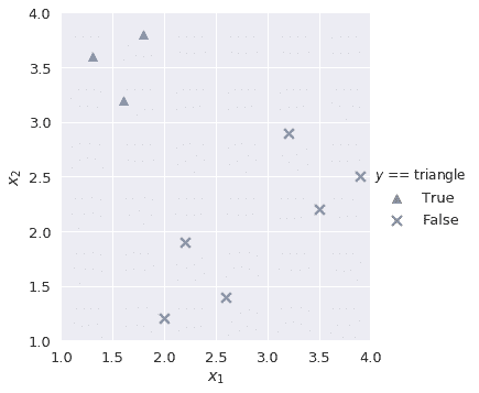我們的目標是構建一個多類分類器，將觀測值標記為$x_1$和$x_2$的給定值`triangle`、`square`或`circle`。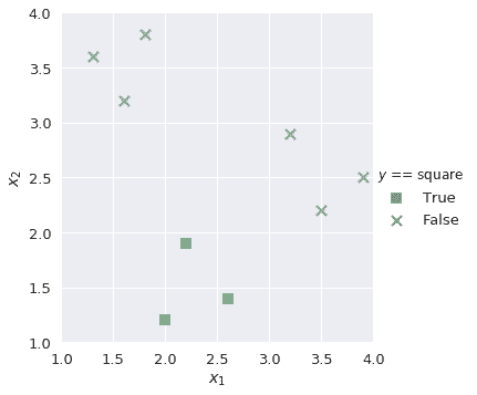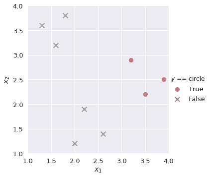首先，我們要構建一個二進制分類器`lr_triangle`，它將觀察結果預測為`triangle`或非`triangle`： ``` plot_binary(shapes, 'triangle') ```  同樣，我們為剩余的類構建二進制分類器`lr_square`和`lr_circle`。 ``` plot_binary(shapes, 'square') ```  ``` plot_binary(shapes, 'circle') ```  我們知道，在邏輯回歸中，乙狀結腸函數的輸出是從 0 到 1 的概率值。為了解決我們的多類分類任務，我們在每個二進制分類器中找到正類的概率，并選擇輸出最高正類概率的類。例如，如果我們有一個具有以下值的新觀察值： | $XY1 $ | $XY2 $ | | --- | --- | | 第 3.2 條 | 2.5 條 | 然后我們的多類分類器將這些值輸入到`lr_triangle`、`lr_square`和`lr_circle`中的每一個。我們提取三個分類器的正類概率： ``` # HIDDEN lr_triangle = LogisticRegression(random_state=42) lr_triangle.fit(shapes[['$x_1$', '$x_2$']], shapes['$y$'] == 'triangle') proba_triangle = lr_triangle.predict_proba([[3.2, 2.5]])[0][1] lr_square = LogisticRegression(random_state=42) lr_square.fit(shapes[['$x_1$', '$x_2$']], shapes['$y$'] == 'square') proba_square = lr_square.predict_proba([[3.2, 2.5]])[0][1] lr_circle = LogisticRegression(random_state=42) lr_circle.fit(shapes[['$x_1$', '$x_2$']], shapes['$y$'] == 'circle') proba_circle = lr_circle.predict_proba([[3.2, 2.5]])[0][1] ``` | `lr_triangle` | `lr_square` | `lr_circle` | | --- | --- | --- | | 0.145748 個 | 0.285079 美元 | 0.497612 個 | 由于`lr_circle`的正類概率是三種概率中最大的，因此我們的多類分類器預測觀察結果是一個圓。 ## 案例研究：IRIS 數據集[?](#Case-Study:-Iris-dataset) IRIS 數據集是一種著名的數據集，在數據科學中經常用于探索機器學習概念。有三類，每類代表一種鳶尾植物： * 剛毛鳶尾 * 雜色鳶尾 * 弗吉尼亞鳶尾 數據集中有四個可用功能： * 萼片長度（厘米） * 萼片寬度（cm） * 花瓣長度（cm） * 花瓣寬度（cm）  我們將創建一個多類分類器，根據上述四個特征預測鳶尾植物的類型。首先，我們讀取數據： ``` iris = pd.read_csv('https://archive.ics.uci.edu/ml/machine-learning-databases/iris/iris.data', header=None, names=['sepal_length', 'sepal_width', 'petal_length', 'petal_width', 'species']) iris ``` | | 萼片長度 | 萼片寬度 | 花瓣長度 | 花瓣寬度 | 物種 | | --- | --- | --- | --- | --- | --- | | 零 | 五點一 | 第 3.5 條 | 一點四 | 0.2 條 | 剛毛鳶尾 | | --- | --- | --- | --- | --- | --- | | 1 個 | 四點九 | 三 | 1.4 | 0.2 | Iris-setosa | | --- | --- | --- | --- | --- | --- | | 二 | 四點七 | 3.2 | 一點三 | 0.2 | Iris-setosa | | --- | --- | --- | --- | --- | --- | | …… | …… | ... | ... | ... | ... | | --- | --- | --- | --- | --- | --- | | 147 個 | 6.5 條 | 3.0 | 五點二 | 二 | 弗吉尼亞鳶尾 | | --- | --- | --- | --- | --- | --- | | 一百四十八 | 六點二 | 三點四 | 五點四 | 二點三 | Iris-virginica | | --- | --- | --- | --- | --- | --- | | 149 個 | 五點九 | 3.0 | 5.1 | 一點八 | Iris-virginica | | --- | --- | --- | --- | --- | --- | 150 行×5 列 ``` X, y = iris.drop('species', axis=1), iris['species'] X_train, X_test, y_train, y_test = train_test_split(X, y, test_size=0.35, random_state=42) ``` 在將數據集劃分為訓練和測試分割之后，我們將多類分類器與我們的訓練數據相匹配。默認情況下，SciKit Learn 的`LogisticRegression`設置`multi_class='ovr'`，它為每個唯一類創建二進制分類器： ``` lr = LogisticRegression(random_state=42) lr.fit(X_train, y_train) ``` ``` LogisticRegression(C=1.0, class_weight=None, dual=False, fit_intercept=True, intercept_scaling=1, max_iter=100, multi_class='ovr', n_jobs=1, penalty='l2', random_state=42, solver='liblinear', tol=0.0001, verbose=0, warm_start=False) ``` 我們對測試數據進行預測，并使用一個混淆矩陣來評估結果。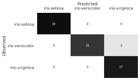 ``` y_pred = lr.predict(X_test) plot_confusion_matrix(y_test, y_pred) ```  混淆矩陣表明，我們的分類器將兩個`Iris-versicolor`觀察結果誤分類為`Iris-virginica`。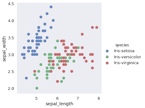在觀察`sepal_length`和`sepal_width`特征時，我們可以假設為什么會發生這種情況： ``` # HIDDEN sns.lmplot(x='sepal_length', y='sepal_width', data=iris, hue='species', fit_reg=False); ```  這兩個特性的`Iris-versicolor`和`Iris-virginica`點重疊。雖然剩下的特性（`petal_width`和`petal_length`）有助于區分這兩個類，但是我們的分類器仍然對這兩個觀察結果進行了錯誤分類。 同樣，在現實世界中，如果兩個類具有相似的特性，則錯誤分類可能很常見。混淆矩陣是有價值的，因為它們幫助我們識別分類器所產生的錯誤，從而洞察為了改進分類器，我們可能需要提取哪些額外的特性。 ## 多標簽分類 另一類分類問題是**多標簽分類**，其中每個觀測可以有多個標簽。文件分類系統就是一個例子：文件可以有積極或消極的情緒，宗教或非宗教的內容，自由或保守的傾向。多標簽問題也可以是多類的；我們可能希望我們的文檔分類系統區分一系列類型，或者識別文檔所用的語言。 我們可以通過簡單地在每一組標簽上訓練一個單獨的分類器來執行多標簽分類。為了標記一個新的點，我們結合了每個分類器的預測。 ## 摘要[?](#Summary) 分類問題在本質上往往是復雜的。有時，這個問題要求我們區分多個類之間的觀察；在其他情況下，我們可能需要為每個觀察指定幾個標簽。我們利用我們對二進制分類器的知識來創建能夠完成這些任務的多類和多標簽分類系統。