# 學生化自舉 > 原文：[https://www.textbook.ds100.org/ch/18/hyp_studentized.html](https://www.textbook.ds100.org/ch/18/hyp_studentized.html) ``` # HIDDEN # Clear previously defined variables %reset -f # Set directory for data loading to work properly import os os.chdir(os.path.expanduser('~/notebooks/18')) ``` ``` # HIDDEN import warnings # Ignore numpy dtype warnings. These warnings are caused by an interaction # between numpy and Cython and can be safely ignored. # Reference: https://stackoverflow.com/a/40846742 warnings.filterwarnings("ignore", message="numpy.dtype size changed") warnings.filterwarnings("ignore", message="numpy.ufunc size changed") import numpy as np import matplotlib.pyplot as plt import pandas as pd import seaborn as sns %matplotlib inline import ipywidgets as widgets from ipywidgets import interact, interactive, fixed, interact_manual import nbinteract as nbi sns.set() sns.set_context('talk') np.set_printoptions(threshold=20, precision=2, suppress=True) pd.options.display.max_rows = 7 pd.options.display.max_columns = 8 pd.set_option('precision', 2) # This option stops scientific notation for pandas # pd.set_option('display.float_format', '{:.2f}'.format) ``` ``` # HIDDEN def df_interact(df, nrows=7, ncols=7): ''' Outputs sliders that show rows and columns of df ''' def peek(row=0, col=0): return df.iloc[row:row + nrows, col:col + ncols] if len(df.columns) <= ncols: interact(peek, row=(0, len(df) - nrows, nrows), col=fixed(0)) else: interact(peek, row=(0, len(df) - nrows, nrows), col=(0, len(df.columns) - ncols)) print('({} rows, {} columns) total'.format(df.shape[0], df.shape[1])) ``` ``` # HIDDEN times = pd.read_csv('ilec.csv')['17.5'] ``` **bootstrap**是我們在數據 8 中了解到的一個過程，我們只能使用一個樣本來估計人口統計。引導的一般步驟如下： * 從人群中抽取相當大的樣本。 * 使用這個樣本，我們用替換品重新取樣，形成相同尺寸的新樣本。 * 我們做了很多次，對每個重采樣進行期望的統計（例如，我們取每個重采樣的中位數）。 在這里，我們得到了許多來自個別重采樣的測試統計數據，從中我們可以形成一個分布。在數據 8 中，我們被教導通過采用引導統計的 2.5%和 97.5%來形成 95%的置信區間。這種用于創建置信區間的引導方法稱為**百分位數引導。**95%置信度意味著，如果我們從總體中提取一個新的樣本并構造一個置信區間，置信區間將包含概率為 0.95 的總體參數。然而，重要的是要注意，從實際數據創建的置信區間只能接近 95%的置信度。特別是在小樣本量的情況下，百分位數引導比期望的置信度要低。 下面，我們選取了一個總體，并為不同樣本大小的總體平均值創建了 1000 個引導 95%的置信區間。Y 軸表示包含實際總體平均值的 1000 個置信區間的分數。注意，在樣本量低于 20 的情況下，小于 90%的置信區間實際上包含總體平均值。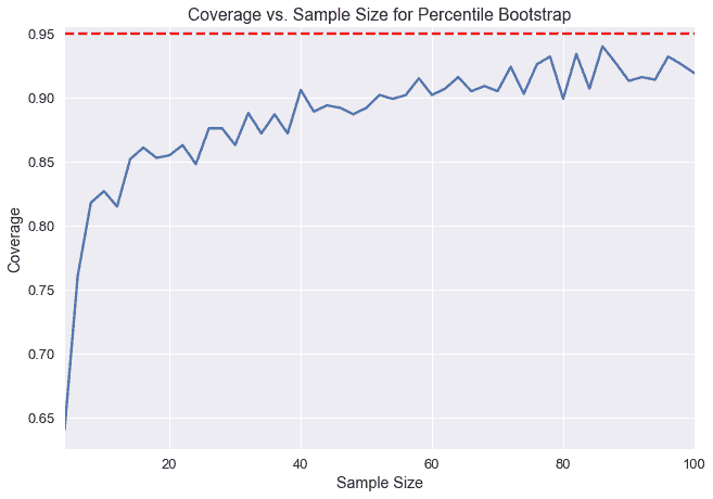  我們可以通過計算我們這里測量的置信度和我們期望的 95%置信度之間的差異來測量 _ 覆蓋誤差 _。我們可以看到，在小樣本量的情況下，百分位數引導的覆蓋率誤差非常高。在本章中，我們將介紹一種新的引導方法，稱為**studentized bootstrap**方法，它具有較低的覆蓋率錯誤，但需要更多的計算。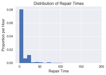 ### 修理次數[?](#Repair-Times) 紐約市公用事業委員會監測該州修理陸地電話服務的響應時間。這些維修時間可能會因維修類型的不同而有所不同。我們對一個特定的 _ 現有本地交換運營商 _ 進行了一次一類維修的維修時間普查，該公司是一家電話公司，在向競爭激烈的本地交換運營商開放市場之前，該公司對固定電話服務擁有區域壟斷權，或者這類公司的法人繼承人。委員會對平均維修時間的估計很感興趣。首先，讓我們看看所有時間的分布。 ``` plt.hist(times, bins=20, normed=True) plt.xlabel('Repair Time') plt.ylabel('Proportion per Hour') plt.title('Distribution of Repair Times'); ```  假設我們要估計修復時間的總體平均值。我們首先需要定義實現這一點所需的主要統計函數。通過對整個人口的統計，我們可以看出實際平均修復時間約為 8.4 小時。 ``` def stat(sample, axis=None): return np.mean(sample, axis=axis) ``` ``` theta = stat(times) theta ``` ``` 8.406145520144333 ``` 現在我們需要定義一個方法，它將返回一個索引列表，這樣我們就可以從原始樣本中重新取樣而不需要替換。 ``` def take_sample(n=10): return np.random.choice(times, size=n, replace=False) ``` 在現實生活中，我們將無法從人群中提取許多樣本（我們使用自舉只能使用一個樣本）。但出于演示目的，我們可以接觸到整個人口，因此我們將采集 1000 個 10 號樣本，并繪制樣本平均值的分布圖。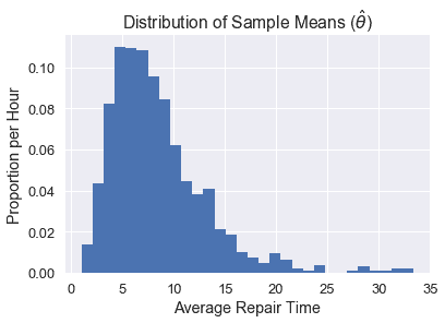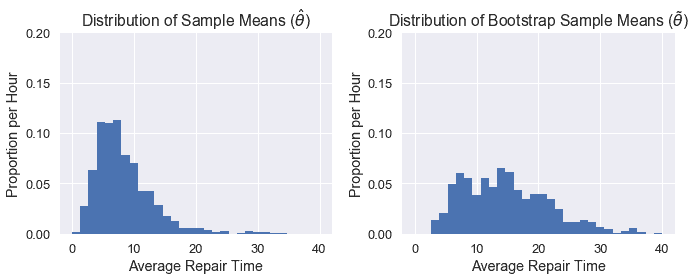 ``` samples_from_pop = 1000 pop_sampling_dist = np.array( [stat(take_sample()) for _ in range(samples_from_pop)] ) plt.hist(pop_sampling_dist, bins=30, normed=True); plt.xlabel('Average Repair Time') plt.ylabel('Proportion per Hour') plt.title(r'Distribution of Sample Means ($\hat{\theta}$)'); ```  我們可以看到，這個分布的中心是~5，并且由于原始數據的分布是傾斜的，所以它是向右傾斜的。 ### 統計分布比較 現在我們可以看看單個引導分布如何與從總體中抽樣的分布相比較。 一般來說，我們的目標是估計我們的人口參數$\theta^*$（在這種情況下，人口的平均修復時間，我們發現是~8.4）。每個單獨的樣本都可以用來計算一個估計的統計，$\hat\theta$（在這種情況下，是單個樣本的平均修復時間）。上面的圖表顯示了我們所稱的 _ 經驗分布 _，它是由人口中許多樣本的估計統計數據計算得出的。但是，對于自舉，我們需要原始樣本（稱為$\tilde\theta$）重新采樣的統計信息。 為了使自舉正常工作，我們希望原始樣本看起來與總體相似，以便重新取樣看起來也與總體相似。如果我們的原始樣本 _ 看起來像人群，那么從重新取樣計算出的平均修復時間分布將類似于直接從人群中提取的樣本的經驗分布。_ 讓我們來看看一個單獨的引導分布將如何顯示。我們可以定義不需要替換的情況下抽取 10 號樣本的方法，并將其引導 1000 次以獲得我們的分布。 ``` bootstrap_reps = 1000 def resample(sample, reps): n = len(sample) return np.random.choice(sample, size=reps * n).reshape((reps, n)) def bootstrap_stats(sample, reps=bootstrap_reps, stat=stat): resamples = resample(sample, reps) return stat(resamples, axis=1) ``` ``` np.random.seed(0) sample = take_sample() plt.hist(bootstrap_stats(sample), bins=30, normed=True) plt.xlabel('Average Repair Time') plt.ylabel('Proportion per Hour') plt.title(r'Distribution of Bootstrap Sample Means ($\tilde{\theta}$)'); ```  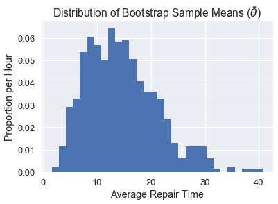正如您所看到的，我們的$\tilde\theta$分布與$\hat\theta$分布不太一樣，這可能是因為我們的原始樣本不像人群。因此，我們的置信區間表現相當差。下面我們可以看到兩個分布的并排比較： ``` plt.figure(figsize=(10, 4)) plt.subplot(121) plt.xlabel('Average Repair Time') plt.ylabel('Proportion per Hour') plt.title(r'Distribution of Sample Means ($\hat{\theta}$)') plt.hist(pop_sampling_dist, bins=30, range=(0, 40), normed=True) plt.ylim((0,0.2)) plt.subplot(122) plt.xlabel('Average Repair Time') plt.ylabel('Proportion per Hour') plt.title(r'Distribution of Bootstrap Sample Means ($\tilde{\theta}$)') plt.hist(bootstrap_stats(sample), bins=30, range=(0, 40), normed=True) plt.ylim((0,0.2)) plt.tight_layout(); ```  ### studentized 自舉[?](#The-Studentized-Bootstrap-Procedure) 正如我們所看到的，百分位數自舉的主要問題是需要更大的樣本量才能真正達到所需的 95%置信度。利用 studentized 自舉，我們可以做更多的計算，以在較小的樣本量下獲得更好的覆蓋率。 研究自舉背后的思想是規范化測試統計的分布$\tilde\theta$以 0 為中心，標準偏差為 1。這將修正原始分布的擴展差和傾斜。為了完成所有這些，我們需要首先進行一些派生。 在百分位數引導過程中，我們生成了許多$\tilde\theta$的值，然后我們將 2.5%和 97.5%作為置信區間。簡言之，我們將這些百分位數稱為$Q_2.5 和$Q_97.5 美元。請注意，這兩個值都來自引導統計信息。 通過這個過程，我們希望實際的人口統計數據在置信區間之間的概率是 95%。換句話說，我們希望實現以下平等： $$\Begin Aligned 0.95&amp；=\Cal P \ Left（Q 2.5 \Leq\Theta ^*\Leq Q 97.5 \ Let Aligned$$ 在這個過程中，我們做了兩個近似：因為我們假設我們的隨機樣本看起來像總體，所以我們用.\that\theta$來近似.\theta^*；因為我們假設一個隨機重采樣看起來像原始樣本，所以我們用.\tilde\theta$來近似.\that\theta$。由于第二個近似值依賴于第一個近似值，所以它們都會在置信區間生成中引入誤差，從而產生我們在圖中看到的覆蓋誤差。 我們的目標是通過標準化我們的統計數據來減少這個錯誤。我們不直接使用我們的計算值$\tilde\theta$，而是使用： $$\begin aligned \frac \tilde \theta-\hat \theta se（\tilde \theta）\end aligned$$ 這將用樣本統計標準化重采樣統計，然后除以重采樣統計的標準偏差（此標準偏差也稱為標準誤差，或 SE）。 整個規范化的統計稱為學生的 t 統計量，所以我們稱這個引導方法為**studentized bootstrap**或**bootstrap-t**方法。 像往常一樣，我們計算了許多重采樣的統計數據，然后取 2.5%和 97.5%分別為$Q_2.5 和$Q_97.5_。因此，我們希望歸一化總體參數位于這些百分位數之間： $$\Begin Aligned 0.95&amp；=\Cal P \ Left（Q 2.5 \Leq\Frac \Hat \Theta-\Theta ^*SE（\Hat \Theta）\Leq Q 97.5 \ Let Aligned$$ 我們現在可以解出$\theta^*$的不等式： $$ \begin{aligned} 0.95 &= {\cal P}\left(q_{2.5} \leq \frac{\hat{\theta} - \theta^*} {SE({\hat{\theta}})} \leq q_{97.5}\right) \\ &= {\cal P}\left(q_{2.5}SE({\hat{\theta}}) \leq {\hat{\theta} - \theta^*} \leq q_{97.5}SE({\hat{\theta}})\right) \\ &= {\cal P}\left(\hat{\theta} - q_{97.5}Se（\Hat \Theta）\Leq \Theta ^*\Leq \Hat \Theta-Q 2.5 Se（\Hat \Theta）\右\端對齊$$ 這意味著我們可以只用$\hat\theta$（原始樣本的測試統計）、$q 2.5 和$q 97.5$（用重采樣計算的標準化統計百分比）和$se（\hat\theta）$（樣本測試統計的標準差）來構造置信區間。最后一個值是通過使用重新取樣測試統計數據的標準偏差來估計的。 因此，要計算 studentized 自舉 CI，我們執行以下過程： 1. 計算樣本上的測試統計數據。 2. 多次引導樣本。 3. 對于每個自舉，重新取樣： 1. 計算$\tilde\theta$，重新取樣的測試統計信息。 2. 計算$SE（\tilde \theta）美元。 3. 計算$Q=\frac \tilde \theta-\hat \theta se（\tilde \theta）$。 4. 使用$\tilde\theta$值的標準偏差估計$se（\hat\theta）$值。 5. 然后計算置信區間：$\Left[\Hat \Theta-Q 97.5 SE（\Hat \Theta），\Hat \Theta-Q 2.5 SE（\Hat \Theta Right）$。 ### 重新取樣統計的標準誤差計算 需要注意的是，$SE（\hat\theta）$是重新采樣測試統計的標準錯誤，它并不總是容易計算，并且依賴于測試統計。對于樣本平均值，$se（\tilde\theta）=\frac \tilde\sigma \sqrt n$，重采樣值的標準差除以樣本大小的平方根。 還要記住，我們必須使用重采樣值來計算$SE（\tilde\theta）$；我們使用示例值來計算$SE（\hat\theta）$。 但是，如果我們的測試統計數據沒有一個分析表達式（就像我們對于樣本平均值的表達式），那么我們需要進行第二級引導。對于每個重采樣，我們再次引導它，并計算每個第二級重采樣（重采樣）的測試統計信息，并使用這些第二級統計信息計算標準偏差。通常，我們會進行大約 50 個二級采樣。 這大大增加了 studentized 引導過程的計算時間。如果我們進行 50 個二級重采樣，整個過程將花費 50 倍的時間，只要我們有一個$SE（\tilde\theta）$的分析表達式。 ### 研究性引導與百分位數引導的比較 為了評估 studentized 和 percentile 引導的權衡，讓我們使用修復時間數據集比較兩種方法的覆蓋率。 ``` plt.hist(times, bins=20, normed=True); plt.xlabel('Repair Time') plt.ylabel('Proportion per Hour') plt.title('Distribution of Repair Times'); ```  我們將從人群中抽取許多樣本，計算每個樣本的百分位置信區間和研究的置信區間，然后計算每個樣本的覆蓋率。我們將對不同的樣本大小重復此操作，以了解每個方法的覆蓋范圍如何隨樣本大小而變化。 我們可以使用`np.percentile`計算以下百分位置信區間： ``` def percentile_ci(sample, reps=bootstrap_reps, stat=stat): stats = bootstrap_stats(sample, reps, stat) return np.percentile(stats, [2.5, 97.5]) ``` ``` np.random.seed(0) sample = take_sample(n=10) percentile_ci(sample) ``` ``` array([ 4.54, 29.56]) ``` 要進行 studentized 引導，我們需要更多的代碼： ``` def studentized_stats(sample, reps=bootstrap_reps, stat=stat): ''' Computes studentized test statistics for the provided sample. Returns the studentized test statistics and the SD of the resample test statistics. ''' # Bootstrap the sample and compute \tilde \theta values resamples = resample(sample, reps) resample_stats = stat(resamples, axis=1) resample_sd = np.std(resample_stats) # Compute SE of \tilde \theta. # Since we're estimating the sample mean, we can use the formula. # Without the formula, we would have to do a second level bootstrap here. resample_std_errs = np.std(resamples, axis=1) / np.sqrt(len(sample)) # Compute studentized test statistics (q values) sample_stat = stat(sample) t_statistics = (resample_stats - sample_stat) / resample_std_errs return t_statistics, resample_sd def studentized_ci(sample, reps=bootstrap_reps, stat=stat): ''' Computes 95% studentized bootstrap CI ''' t_statistics, resample_sd = studentized_stats(sample, reps, stat) lower, upper = np.percentile(t_statistics, [2.5, 97.5]) sample_stat = stat(sample) return (sample_stat - resample_sd * upper, sample_stat - resample_sd * lower) ``` ``` np.random.seed(0) sample = take_sample(n=10) studentized_ci(sample) ``` ``` (4.499166906400612, 59.03291210887363) ``` 現在所有內容都寫出來了，我們可以比較兩種方法的覆蓋范圍，因為樣本大小從 4 增加到 100。 ``` def coverage(cis, parameter=theta): return ( np.count_nonzero([lower < parameter < upper for lower, upper in cis]) / len(cis) ) ``` ``` def run_trials(sample_sizes): np.random.seed(0) percentile_coverages = [] studentized_coverages = [] for n in sample_sizes: samples = [take_sample(n) for _ in range(samples_from_pop)] percentile_cis = [percentile_ci(sample) for sample in samples] studentized_cis = [studentized_ci(sample) for sample in samples] percentile_coverages.append(coverage(percentile_cis)) studentized_coverages.append(coverage(studentized_cis)) return pd.DataFrame({ 'percentile': percentile_coverages, 'studentized': studentized_coverages, }, index=sample_sizes) ``` ``` %%time trials = run_trials(np.arange(4, 101, 2)) ``` ``` CPU times: user 1min 52s, sys: 1.08 s, total: 1min 53s Wall time: 1min 57s ``` ``` trials.plot() plt.axhline(0.95, c='red', linestyle='--', label='95% coverage') plt.legend() plt.xlabel('Sample Size') plt.ylabel('Coverage') plt.title('Coverage vs. 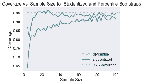Sample Size for Studentized and Percentile Bootstraps'); ```  如我們所見，在較小的樣本量下，studentized 引導具有更好的覆蓋范圍。 ## 摘要[?](#Summary) 大多數情況下，研究的引導比百分位引導更好，特別是如果我們只有一個小樣本開始。我們通常希望在樣本量較小或原始數據傾斜時使用此方法。主要的缺點是它的計算時間，如果$SE（\tilde\theta）$不容易計算，它會被進一步放大。