# L2 正則化：嶺回歸 > 原文：[https://www.bookbookmark.ds100.org/ch/16/reg_ridge.html](https://www.bookbookmark.ds100.org/ch/16/reg_ridge.html) ``` # HIDDEN # Clear previously defined variables %reset -f # Set directory for data loading to work properly import os os.chdir(os.path.expanduser('~/notebooks/16')) ``` ``` # HIDDEN import warnings # Ignore numpy dtype warnings. These warnings are caused by an interaction # between numpy and Cython and can be safely ignored. # Reference: https://stackoverflow.com/a/40846742 warnings.filterwarnings("ignore", message="numpy.dtype size changed") warnings.filterwarnings("ignore", message="numpy.ufunc size changed") import numpy as np import matplotlib.pyplot as plt import pandas as pd import seaborn as sns %matplotlib inline import ipywidgets as widgets from ipywidgets import interact, interactive, fixed, interact_manual import nbinteract as nbi sns.set() sns.set_context('talk') np.set_printoptions(threshold=20, precision=2, suppress=True) pd.options.display.max_rows = 7 pd.options.display.max_columns = 8 pd.set_option('precision', 2) # This option stops scientific notation for pandas # pd.set_option('display.float_format', '{:.2f}'.format) ``` ``` # HIDDEN def df_interact(df, nrows=7, ncols=7): ''' Outputs sliders that show rows and columns of df ''' def peek(row=0, col=0): return df.iloc[row:row + nrows, col:col + ncols] if len(df.columns) <= ncols: interact(peek, row=(0, len(df) - nrows, nrows), col=fixed(0)) else: interact(peek, row=(0, len(df) - nrows, nrows), col=(0, len(df.columns) - ncols)) print('({} rows, {} columns) total'.format(df.shape[0], df.shape[1])) ``` ``` # HIDDEN df = pd.read_csv('water_large.csv') ``` ``` # HIDDEN from collections import namedtuple Curve = namedtuple('Curve', ['xs', 'ys']) def flatten(seq): return [item for subseq in seq for item in subseq] def make_curve(clf, x_start=-50, x_end=50): xs = np.linspace(x_start, x_end, num=100) ys = clf.predict(xs.reshape(-1, 1)) return Curve(xs, ys) def plot_data(df=df, ax=plt, **kwargs): ax.scatter(df.iloc[:, 0], df.iloc[:, 1], s=50, **kwargs) def plot_curve(curve, ax=plt, **kwargs): ax.plot(curve.xs, curve.ys, **kwargs) def plot_curves(curves, cols=2, labels=None): if labels is None: labels = [f'Deg {deg} poly' for deg in degrees] rows = int(np.ceil(len(curves) / cols)) fig, axes = plt.subplots(rows, cols, figsize=(10, 8), sharex=True, sharey=True) for ax, curve, label in zip(flatten(axes), curves, labels): plot_data(ax=ax, label='Training data') plot_curve(curve, ax=ax, label=label) ax.set_ylim(-5e10, 170e10) ax.legend() # add a big axes, hide frame fig.add_subplot(111, frameon=False) # hide tick and tick label of the big axes plt.tick_params(labelcolor='none', top='off', bottom='off', left='off', right='off') plt.grid(False) plt.title('Polynomial Regression') plt.xlabel('Water Level Change (m)') plt.ylabel('Water Flow (Liters)') plt.tight_layout() ``` ``` # HIDDEN def coefs(clf): reg = clf.named_steps['reg'] return np.append(reg.intercept_, reg.coef_) def coef_table(clf): vals = coefs(clf) return (pd.DataFrame({'Coefficient Value': vals}) .rename_axis('degree')) ``` ``` # HIDDEN X = df.iloc[:, [0]].as_matrix() y = df.iloc[:, 1].as_matrix() degrees = [1, 2, 8, 12] clfs = [Pipeline([('poly', PolynomialFeatures(degree=deg, include_bias=False)), ('reg', LinearRegression())]) .fit(X, y) for deg in degrees] curves = [make_curve(clf) for clf in clfs] alphas = [0.01, 0.1, 1.0, 10.0] ridge_clfs = [Pipeline([('poly', PolynomialFeatures(degree=deg, include_bias=False)), ('reg', RidgeCV(alphas=alphas, normalize=True))]) .fit(X, y) for deg in degrees] ridge_curves = [make_curve(clf) for clf in ridge_clfs] ``` 在本節中，我們將介紹$L_2$正則化，這是一種在成本函數中懲罰大權重以降低模型方差的方法。我們簡要回顧了線性回歸，然后引入正則化作為對成本函數的修正。 為了進行最小二乘線性回歸，我們使用以下模型： $$ f_\hat{\theta}(x) = \hat{\theta} \cdot x $$ 我們通過最小化均方誤差成本函數來擬合模型： $$ \begin{aligned} L(\hat{\theta}, X, y) &= \frac{1}{n} \sum_{i}^n(y_i - f_\hat{\theta} (X_i))^2\\ \end{aligned} $$ 在上述定義中，$x$表示$n 乘以 p$數據矩陣，$x$表示$x$的一行，$y$表示觀察到的結果，$that \theta$表示模型權重。 ## 二級規范化定義 要將$L_2$正則化添加到模型中，我們修改上面的成本函數： $$ \begin{aligned} L(\hat{\theta}, X, y) &= \frac{1}{n} \sum_{i}(y_i - f_\hat{\theta} (X_i))^2 + \lambda \sum_{j = 1}^{p} \hat{\theta_j}^2 \end{aligned} $$ 請注意，上面的成本函數與前面的相同，加上$L_2$Regularization$\lambda\sum_j=1 ^ p \hat \theta_j ^2$term。本術語中的總和是每種型號重量的平方和，即$\Hat \Theta、\Hat \Theta、\Ldots、\Hat \Theta P。這個術語還引入了一個新的標量模型參數$\lambda$來調整正則化懲罰。 如果$\that \theta$中的值遠離 0，正則化術語會導致成本增加。加入正則化后，最優模型權重將損失和正則化懲罰的組合最小化，而不是只考慮損失。由于得到的模型權重在絕對值上趨向于較小，因此該模型具有較低的方差和較高的偏差。 使用$l_2$正則化和線性模型以及均方誤差成本函數，通常也被稱為**嶺回歸**。 ### 正則化參數[?](#The-Regularization-Parameter) 正則化參數$\lambda$控制正則化懲罰。一個小的$\lambda$會導致一個小的懲罰，如果$\lambda=0$正則化術語也是$0$并且成本根本沒有正則化。 一個大的$\lambda$術語會導致一個大的懲罰，因此是一個更簡單的模型。增加$\lambda$會減少方差并增加模型的偏差。我們使用交叉驗證來選擇$\lambda$的值，以最小化驗證錯誤。 **關于`scikit-learn`中正則化的說明：** `scikit-learn`提供了內置正則化的回歸模型。例如，要進行嶺回歸，可以使用[`sklearn.linear_model.Ridge`](http://scikit-learn.org/stable/modules/generated/sklearn.linear_model.Ridge.html)回歸模型。注意，`scikit-learn`模型調用正則化參數`alpha`而不是$\lambda$。 `scikit-learn`方便地提供了規范化模型，這些模型執行交叉驗證以選擇一個好的值$\lambda$。例如，[`sklearn.linear_model.RidgeCV`](http://scikit-learn.org/stable/modules/generated/sklearn.linear_model.RidgeCV.html#sklearn.linear_model.RidgeCV)允許用戶輸入正則化參數值，并自動使用交叉驗證來選擇驗證錯誤最小的參數值。 ### 偏壓項排除 注意，偏差項$\theta_$不包括在正則化項的總和中。我們不懲罰偏倚項，因為增加偏倚項不會增加模型的方差。偏倚項只會將所有預測值移動一個常量。 ### 數據規范化 注意，正則化術語$\lambda\sum_j=1 ^ p \that \theta ^2$對每個\theta j 2$的懲罰是相等的。但是，每個$\hat \theta j 的效果因數據本身而異。在添加 8 次多項式特征后，考慮水流數據集的這一部分： ``` # HIDDEN pd.DataFrame(clfs[2].named_steps['poly'].transform(X[:5]), columns=[f'deg_{n}_feat' for n in range(8)]) ``` | | deg_0_ 專長 | deg_1_ 專長 | …… | deg_6_ 專長 | deg_7_ 專長 | | --- | --- | --- | --- | --- | --- | | 零 | -15 | 二百五十三點九八 | …… | -261095791.08 元 | 4161020472.12 年 | | --- | --- | --- | --- | --- | --- | | 1 個 | -27.15 | 八百四十九點九零 | ... | -17897014961.65 | 521751305227.70 | | --- | --- | --- | --- | --- | --- | | 二 | 三十六點一九 | 1309.68 號 | ... | 81298431147.09 | 2942153527269.12 | | --- | --- | --- | --- | --- | --- | | 三 | 三十七點四九 | 1405.66 元 | ... | 104132296999.30 | 3904147586408.71 | | --- | --- | --- | --- | --- | --- | | 四 | -41.06 | 2309.65 美元 | ... 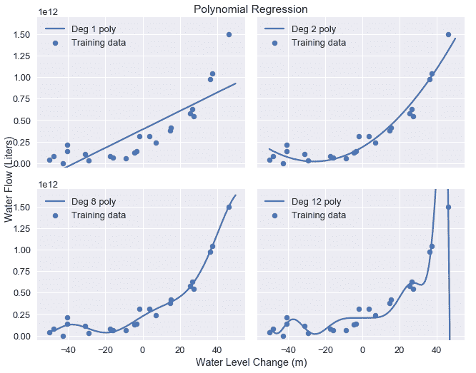| -592123531634.12 | 28456763821657.78 | | --- | --- | --- | --- | --- | --- | 5 行×8 列 我們可以看到 7 次多項式的特征值比 1 次多項式的特征值大得多。這意味著 7 級特征的大型模型權重對預測的影響遠大于 1 級特征的大型模型權重。如果我們直接對這些數據應用正則化，正則化懲罰將不成比例地降低低階特征的模型權重。在實際應用中，由于對預測影響較大的特征不受影響，即使采用正則化，也往往導致模型方差較大。 為了解決這個問題，我們 _ 通過減去平均值并將每一列中的值縮放到-1 和 1 之間來規范化 _ 每個數據列。在`scikit-learn`中，大多數回歸模型允許使用`normalize=True`進行初始化，以便在擬合前規范化數據。 另一種類似的技術是 _ 標準化 _ 數據列，方法是減去平均值并除以每個數據列的標準偏差。 ## 使用嶺回歸 我們以前使用多項式特征來擬合 2、8 和 12 度多項式以獲得水流數據。原始數據和結果模型預測在下面重復。 ``` # HIDDEN df ``` | | 水位變化 | 水流 | | --- | --- | --- | | 0 | -15.94 | 60422330445.52 號 | | --- | --- | --- | | 1 | -29.15 | 33214896575.60 元 | | --- | --- | --- | | 2 | 36.19 | 972706380901.06 | | --- | --- | --- | | ... | ... | ... | | --- | --- | --- | | 20 個 | 七點零九 | 236352046523.78 個 | | --- | --- | --- | | 21 歲 | 四十六點二八 | 149425638186.73 | | --- | --- | --- | | 二十二 | 十四點六一 | 378146284247.97 美元 | | --- | --- | --- | 23 行×2 列 ``` # HIDDEN plot_curves(curves) ```  為了進行嶺回歸，我們首先從數據中提取數據矩陣和結果向量： ``` X = df.iloc[:, [0]].as_matrix() y = df.iloc[:, 1].as_matrix() print('X: ') print(X) print() print('y: ') print(y) ``` ``` X: [[-15.94] [-29.15] [ 36.19] ... [ 7.09] [ 46.28] [ 14.61]] y: [6.04e+10 3.32e+10 9.73e+11 ... 2.36e+11 1.49e+12 3.78e+11] ``` 然后，我們對`X`應用 12 次多項式變換： ``` from sklearn.preprocessing import PolynomialFeatures # We need to specify include_bias=False since sklearn's classifiers # automatically add the intercept term. X_poly_8 = PolynomialFeatures(degree=8, include_bias=False).fit_transform(X) print('First two rows of transformed X:') print(X_poly_8[0:2]) ``` ``` First two rows of transformed X: [[-1.59e+01 2.54e+02 -4.05e+03 6.45e+04 -1.03e+06 1.64e+07 -2.61e+08 4.16e+09] [-2.92e+01 8.50e+02 -2.48e+04 7.22e+05 -2.11e+07 6.14e+08 -1.79e+10 5.22e+11]] ``` 我們指定了`scikit-learn`將使用交叉驗證從中選擇的`alpha`值，然后使用`RidgeCV`分類器來匹配轉換的數據。 ``` from sklearn.linear_model import RidgeCV alphas = [0.01, 0.1, 1.0, 10.0] # Remember to set normalize=True to normalize data clf = RidgeCV(alphas=alphas, normalize=True).fit(X_poly_8, y) # Display the chosen alpha value: clf.alpha_ ``` ``` 0.1 ``` 最后，我們在正則化的 8 階分類器旁邊繪制基本 8 階多項式分類器的模型預測： ``` # HIDDEN fig = plt.figure(figsize=(10, 5)) plt.subplot(121) plot_data() plot_curve(curves[2]) plt.title('Base degree 8 polynomial') plt.subplot(122) plot_data() plot_curve(ridge_curves[2]) plt.title('Regularized degree 8 polynomial') plt.tight_layout() ```  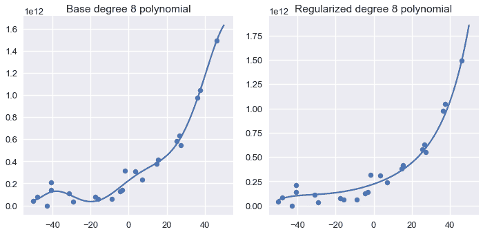我們可以看到，正則化多項式比基階 8 多項式更平滑，并且仍然捕獲了數據中的主要趨勢。 比較非正則化和正則化模型的系數，發現嶺回歸有利于將模型權重放在較低階多項式項上： ``` # HIDDEN base = coef_table(clfs[2]).rename(columns={'Coefficient Value': 'Base'}) ridge = coef_table(ridge_clfs[2]).rename(columns={'Coefficient Value': 'Regularized'}) pd.options.display.max_rows = 20 display(base.join(ridge)) pd.options.display.max_rows = 7 ``` | | 底座 | 正規化 | | --- | --- | --- | | 度 | | | | --- | --- | --- | | 0 | 225782472111.94 美元 | 221063525725.23 | | --- | --- | --- | | 1 | 13115217770.78 號 | 6846139065.96 美元 | | --- | --- | --- | | 2 | -144725749.98 美元 | 146158037.96 號 | | --- | --- | --- | | 3 | -10355082.91 元 | 193090.04 年 | | --- | --- | --- | | 4 | 567935.23 元 | 38240.62 元 | | --- | --- | --- | | 5 個 | 9805.14 年 | 五百六十四點二一 | | --- | --- | --- | | 六 | -249.64 條 | 七點二五 | | --- | --- | --- | | 七 | -2.09 | 零點一八 | | --- | --- | --- | | 8 個 | 零點零三 | 零 | | --- | --- | --- | 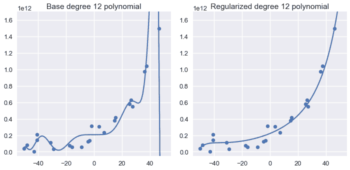重復 12 次多項式特征的過程會得到類似的結果： ``` # HIDDEN fig = plt.figure(figsize=(10, 5)) plt.subplot(121) plot_data() plot_curve(curves[3]) plt.title('Base degree 12 polynomial') plt.ylim(-5e10, 170e10) plt.subplot(122) plot_data() plot_curve(ridge_curves[3]) plt.title('Regularized degree 12 polynomial') plt.ylim(-5e10, 170e10) plt.tight_layout() ```  增加正則化參數會使模型變得越來越簡單。下圖顯示了將正則化量從 0.001 增加到 100.0 的效果。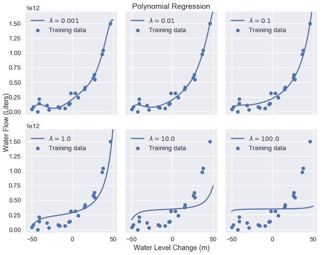 ``` # HIDDEN alphas = [0.001, 0.01, 0.1, 1.0, 10.0, 100.0] alpha_clfs = [Pipeline([ ('poly', PolynomialFeatures(degree=12, include_bias=False)), ('reg', Ridge(alpha=alpha, normalize=True))] ).fit(X, y) for alpha in alphas] alpha_curves = [make_curve(clf) for clf in alpha_clfs] labels = [f'$\\lambda = {alpha}$' for alpha in alphas] plot_curves(alpha_curves, cols=3, labels=labels) ```  如我們所見，增加正則化參數會增加模型的偏差。如果我們的參數太大，模型就會變成一個常量模型，因為任何非零的模型權重都會受到嚴重懲罰。 ## 摘要[?](#Summary) 使用$L_2$正則化可以通過懲罰大型模型權重來調整模型偏差和方差。$L_2$最小二乘線性回歸的正則化也被更常見的名稱嶺回歸所知。使用正則化添加了一個額外的模型參數$\lambda$，我們使用交叉驗證進行調整。