# 凸性 > 原文：[https://www.bookbookmark.ds100.org/ch/11/gradient_convexity.html](https://www.bookbookmark.ds100.org/ch/11/gradient_convexity.html) ``` # HIDDEN # Clear previously defined variables %reset -f # Set directory for data loading to work properly import os os.chdir(os.path.expanduser('~/notebooks/11')) ``` ``` # HIDDEN import warnings # Ignore numpy dtype warnings. These warnings are caused by an interaction # between numpy and Cython and can be safely ignored. # Reference: https://stackoverflow.com/a/40846742 warnings.filterwarnings("ignore", message="numpy.dtype size changed") warnings.filterwarnings("ignore", message="numpy.ufunc size changed") import numpy as np import matplotlib.pyplot as plt import pandas as pd import seaborn as sns %matplotlib inline import ipywidgets as widgets from ipywidgets import interact, interactive, fixed, interact_manual import nbinteract as nbi sns.set() sns.set_context('talk') np.set_printoptions(threshold=20, precision=2, suppress=True) pd.options.display.max_rows = 7 pd.options.display.max_columns = 8 pd.set_option('precision', 2) # This option stops scientific notation for pandas # pd.set_option('display.float_format', '{:.2f}'.format) ``` ``` # HIDDEN tips = sns.load_dataset('tips') tips['pcttip'] = tips['tip'] / tips['total_bill'] * 100 ``` ``` # HIDDEN def mse(theta, y_vals): return np.mean((y_vals - theta) ** 2) def abs_loss(theta, y_vals): return np.mean(np.abs(y_vals - theta)) def quartic_loss(theta, y_vals): return np.mean(1/5000 * (y_vals - theta + 12) * (y_vals - theta + 23) * (y_vals - theta - 14) * (y_vals - theta - 15) + 7) def grad_quartic_loss(theta, y_vals): return -1/2500 * (2 *(y_vals - theta)**3 + 9*(y_vals - theta)**2 - 529*(y_vals - theta) - 327) def plot_loss(y_vals, xlim, loss_fn): thetas = np.arange(xlim[0], xlim[1] + 0.01, 0.05) losses = [loss_fn(theta, y_vals) for theta in thetas] plt.figure(figsize=(5, 3)) plt.plot(thetas, losses, zorder=1) plt.xlim(*xlim) plt.title(loss_fn.__name__) plt.xlabel(r'$ \theta $') plt.ylabel('Loss') def plot_theta_on_loss(y_vals, theta, loss_fn, **kwargs): loss = loss_fn(theta, y_vals) default_args = dict(label=r'$ \theta $', zorder=2, s=200, c=sns.xkcd_rgb['green']) plt.scatter([theta], [loss], **{**default_args, **kwargs}) def plot_connected_thetas(y_vals, theta_1, theta_2, loss_fn, **kwargs): plot_theta_on_loss(y_vals, theta_1, loss_fn) plot_theta_on_loss(y_vals, theta_2, loss_fn) loss_1 = loss_fn(theta_1, y_vals) loss_2 = loss_fn(theta_2, y_vals) plt.plot([theta_1, theta_2], [loss_1, loss_2]) ``` ``` # HIDDEN def plot_one_gd_iter(y_vals, theta, loss_fn, grad_loss, alpha=2.5): new_theta = theta - alpha * grad_loss(theta, y_vals) plot_loss(pts, (-23, 25), loss_fn) plot_theta_on_loss(pts, theta, loss_fn, c='none', edgecolor=sns.xkcd_rgb['green'], linewidth=2) plot_theta_on_loss(pts, new_theta, loss_fn) print(f'old theta: {theta}') print(f'new theta: {new_theta[0]}') ``` 梯度下降提供了一種最小化函數的一般方法。我們觀察到 Huber 損耗，當函數的最小值難以解析地找到時，梯度下降特別有用。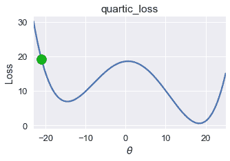 ## 梯度下降找到局部最小值[?](#Gradient-Descent-Finds-Local-Minima) 不幸的是，梯度下降并不總是找到全局最小化的$\theta$。考慮使用下面的損失函數的初始$\theta=-21$進行以下梯度下降運行。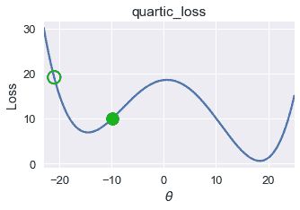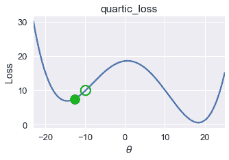 ``` # HIDDEN pts = np.array([0]) plot_loss(pts, (-23, 25), quartic_loss) plot_theta_on_loss(pts, -21, quartic_loss) ```  ``` # HIDDEN plot_one_gd_iter(pts, -21, quartic_loss, grad_quartic_loss) ``` ``` old theta: -21 new theta: -9.944999999999999 ```  ``` # HIDDEN plot_one_gd_iter(pts, -9.9, quartic_loss, grad_quartic_loss) ``` ``` old theta: -9.9 new theta: -12.641412 ```  ``` # HIDDEN plot_one_gd_iter(pts, -12.6, quartic_loss, grad_quartic_loss) ``` ``` old theta: -12.6 new theta: -14.162808 ```  ``` # HIDDEN 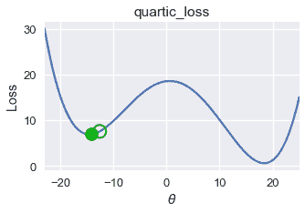plot_one_gd_iter(pts, -14.2, quartic_loss, grad_quartic_loss) ``` ``` old theta: -14.2 new theta: -14.497463999999999 ```  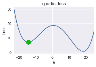在這個損失函數和$theta$值上，梯度下降收斂到$theta=-14.5$，產生大約 8 的損失。但是，這個損失函數的全局最小值是$\theta=18$，相當于幾乎為零的損失。從這個例子中，我們觀察到梯度下降發現了一個局部最小值 _，它可能不一定具有與 _ 全局最小值 _ 相同的損失。_ 幸運的是，許多有用的損失函數具有相同的局部和全局最小值。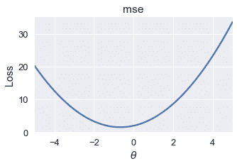考慮常見的均方誤差損失函數，例如： ``` # HIDDEN pts = np.array([-2, -1, 1]) plot_loss(pts, (-5, 5), mse) ```  在這個損失函數上以適當的學習速率進行梯度下降，總是會找到全局最優的$\theta$，因為唯一的局部最小值也是全局最小值。 平均絕對誤差有時有多個局部極小值。然而，所有的局部最小值產生的損失可能是全球最低的。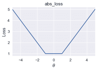 ``` # HIDDEN pts = np.array([-1, 1]) plot_loss(pts, (-5, 5), abs_loss) ```  在這個損失函數上，梯度下降將收斂到$[-1，1]$范圍內的一個局部極小值。由于所有這些局部極小值都具有此函數可能的最小損失，因此梯度下降仍將返回一個最優選擇$\theta$。 ## 凸性的定義 對于某些函數，任何局部最小值也是全局最小值。這組函數被稱為**凸函數**，因為它們向上彎曲。對于常數模型，MSE、MAE 和 Huber 損耗都是凸的。 在適當的學習速率下，梯度下降找到凸損失函數的全局最優值。由于這個有用的性質，我們更喜歡使用凸損失函數來擬合我們的模型，除非我們有充分的理由不這樣做。 形式上，函數$f$是凸的，前提是并且僅當它滿足以下不等式時，對于所有可能的函數輸入$a$和$b$，對于[0，1]$中的所有$t\ $$tf(a) + (1-t)f(b) \geq f(ta + (1-t)b)$$ 這個不等式表明，連接函數兩點的所有線必須位于函數本身之上或之上。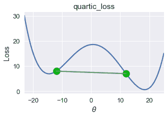對于本節開頭的損失函數，我們可以很容易地找到出現在圖下面的一條線： ``` # HIDDEN pts = np.array([0]) plot_loss(pts, (-23, 25), quartic_loss) plot_connected_thetas(pts, -12, 12, quartic_loss) ```  因此，這個損失函數是非凸的。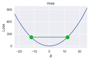 對于 mse，連接圖上兩點的所有線都顯示在圖的上方。我們在下面畫一條這樣的線。 ``` # HIDDEN pts = np.array([0]) plot_loss(pts, (-23, 25), mse) plot_connected_thetas(pts, -12, 12, mse) ```  凸性的數學定義給了我們一個精確的方法來確定函數是否是凸的。在這本教科書中，我們將省略凸性的數學證明，而是說明所選的損失函數是否凸。 ## 摘要[?](#Summary) 對于凸函數，任何局部極小值也是全局極小值。這種有用的性質使得梯度下降能夠有效地找到給定損失函數的全局最優模型參數。當非凸損失函數的梯度下降收斂到局部極小值時，這些局部極小值不能保證是全局最優的。