# 預測冰淇淋評級 > 原文：[https://www.textbook.ds100.org/ch/14/feature_polynomy.html](https://www.textbook.ds100.org/ch/14/feature_polynomy.html) ``` # HIDDEN # Clear previously defined variables %reset -f # Set directory for data loading to work properly import os os.chdir(os.path.expanduser('~/notebooks/14')) ``` ``` # HIDDEN import warnings # Ignore numpy dtype warnings. These warnings are caused by an interaction # between numpy and Cython and can be safely ignored. # Reference: https://stackoverflow.com/a/40846742 warnings.filterwarnings("ignore", message="numpy.dtype size changed") warnings.filterwarnings("ignore", message="numpy.ufunc size changed") import numpy as np import matplotlib.pyplot as plt import pandas as pd import seaborn as sns %matplotlib inline import ipywidgets as widgets from ipywidgets import interact, interactive, fixed, interact_manual import nbinteract as nbi sns.set() sns.set_context('talk') np.set_printoptions(threshold=20, precision=2, suppress=True) pd.options.display.max_rows = 7 pd.options.display.max_columns = 8 pd.set_option('precision', 2) # This option stops scientific notation for pandas # pd.set_option('display.float_format', '{:.2f}'.format) ``` ``` # HIDDEN def df_interact(df, nrows=7, ncols=7): ''' Outputs sliders that show rows and columns of df ''' def peek(row=0, col=0): return df.iloc[row:row + nrows, col:col + ncols] if len(df.columns) <= ncols: interact(peek, row=(0, len(df) - nrows, nrows), col=fixed(0)) else: interact(peek, row=(0, len(df) - nrows, nrows), col=(0, len(df.columns) - ncols)) print('({} rows, {} columns) total'.format(df.shape[0], df.shape[1])) ``` ``` # HIDDEN # To determine which columns to regress # ice_orig = pd.read_csv('icecream_orig.csv') # cols = ['aerated', 'afterfeel', 'almond', 'buttery', 'color', 'cooling', # 'creamy', 'doughy', 'eggy', 'fat', 'fat_level', 'fatty', 'hardness', # 'ice_crystals', 'id', 'liking_flavor', 'liking_texture', 'melt_rate', # 'melting_rate', 'milky', 'sugar', 'sugar_level', 'sweetness', # 'tackiness', 'vanilla'] # melted = ice_orig.melt(id_vars='overall', value_vars=cols, var_name='type') # sns.lmplot(x='value', y='overall', col='type', col_wrap=5, data=melted, # sharex=False, fit_reg=False) ``` 假設我們正在嘗試創造新的，流行的冰淇淋口味。我們對以下回歸問題很感興趣：考慮到冰淇淋的甜味，預測它的總體口味等級為 7。 ``` ice = pd.read_csv('icecream.csv') ice ``` | | 甜度 | 總體的 | | --- | --- | --- | | 零 | 第 4.1 條 | 三點九 | | --- | --- | --- | | 1 個 | 六點九 | 五點四 | | --- | --- | --- | | 二 | 八點三 | 五點八 | | --- | --- | --- | | …… | …… | ... 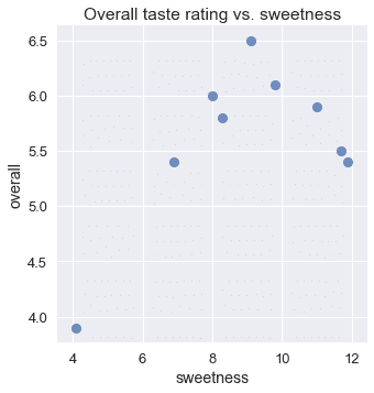| | --- | --- | --- | | 六 | 11.0 條 | 五點九 | | --- | --- | --- | | 七 | 十一點七 | 第 5.5 條 | | --- | --- | --- | | 8 個 | 十一點九 | 5.4 | | --- | --- | --- | 9 行×2 列 雖然我們預計不夠甜的冰淇淋口味將獲得較低的評級，但我們也預計過于甜的冰淇淋口味也將獲得較低的評級。這反映在整體評分和甜度的散點圖中： ``` # HIDDEN sns.lmplot(x='sweetness', y='overall', data=ice, fit_reg=False) plt.title('Overall taste rating vs. 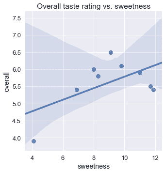sweetness'); ```  不幸的是，僅僅一個線性模型不能考慮這種增加然后減少的行為；在一個線性模型中，整體評級只能隨著甜度單調地增加或減少。我們可以看到，使用線性回歸會導致擬合不良。 ``` # HIDDEN sns.lmplot(x='sweetness', y='overall', data=ice) plt.title('Overall taste rating vs. sweetness'); ```  對于這個問題，一個有用的方法是擬合多項式曲線而不是直線。這樣一條曲線可以讓我們模擬這樣一個事實：總體評分隨著甜味的增加而增加，直到某一點，然后隨著甜味的增加而降低。 使用特征工程技術，我們可以簡單地在數據中添加新的列，以使用線性模型進行多項式回歸。 ## 多項式特征 回想一下，在線性回歸中，我們為數據矩陣$x$的每一列擬合一個權重。在這種情況下，我們的矩陣$X$包含兩列：一列所有列和甜度。 ``` # HIDDEN from sklearn.preprocessing import PolynomialFeatures first_X = PolynomialFeatures(degree=1).fit_transform(ice[['sweetness']]) pd.DataFrame(data=first_X, columns=['bias', 'sweetness']) ``` | | 偏倚 | sweetness | | --- | --- | --- | | 0 | 1.0 條 | 4.1 | | --- | --- | --- | | 1 | 1.0 | 6.9 | | --- | --- | --- | | 2 | 1.0 | 8.3 | | --- | --- | --- | | ... | ... | ... | | --- | --- | --- | | 6 | 1.0 | 11.0 | | --- | --- | --- | | 7 | 1.0 | 11.7 | | --- | --- | --- | | 8 | 1.0 | 11.9 | | --- | --- | --- | 9 rows × 2 columns 因此，我們的模型是： $$ f_\hat{\theta} (x) = \hat{\theta_0} + \hat{\theta_1} \cdot \text{sweetness} $$ 我們可以用$x$創建一個新列，其中包含甜度的平方值。 ``` # HIDDEN second_X = PolynomialFeatures(degree=2).fit_transform(ice[['sweetness']]) pd.DataFrame(data=second_X, columns=['bias', 'sweetness', 'sweetness^2']) ``` | | bias | sweetness | 甜度^2 | | --- | --- | --- | --- | | 0 | 1.0 | 4.1 | 16.81 元 | | --- | --- | --- | --- | | 1 | 1.0 | 6.9 | 四十七點六一 | | --- | --- | --- | --- | | 2 | 1.0 | 8.3 | 六十八點八九 | | --- | --- | --- | --- | | ... | ... | ... | ... | | --- | --- | --- | --- | | 6 | 1.0 | 11.0 | 一百二十一 | | --- | --- | --- | --- | | 7 | 1.0 | 11.7 | 一百三十六點八九 | | --- | --- | --- | --- | | 8 | 1.0 | 11.9 | 一百四十一點六一 | | --- | --- | --- | --- | 9 行×3 列 由于我們的模型為其輸入矩陣的每列學習一個權重，因此我們的模型將成為： $$ f_\hat{\theta} (x) = \hat{\theta_0} + \hat{\theta_1} \cdot \text{sweetness} + \hat{\theta_2} \cdot \text{sweetness}^2 $$ 我們的模型現在與我們的數據擬合二次多項式。我們可以通過為“$\text sweetness ^3$”、“$\text sweetness ^4$”等添加列來輕松適應更高程度的多項式。 注意，這個模型仍然是一個線性模型，因為它的參數是**線性的，每個$\hat \theta i$都是一個階數的標量值。但是，該模型在其特性**中是**多項式，因為其輸入數據包含另一列的多項式轉換列。** ## 多項式回歸 為了進行多項式回歸，我們使用具有多項式特征的線性模型。因此，我們從`scikit-learn`導入[`LinearRegression`](http://scikit-learn.org/stable/modules/generated/sklearn.linear_model.LinearRegression.html#sklearn.linear_model.LinearRegression)模型和[`PolynomialFeatures`](http://scikit-learn.org/stable/modules/generated/sklearn.preprocessing.PolynomialFeatures.html#sklearn.preprocessing.PolynomialFeatures)轉換。 ``` from sklearn.linear_model import LinearRegression from sklearn.preprocessing import PolynomialFeatures ``` 我們的原始數據矩陣$x$包含以下值。請記住，我們包含的列和行標簽僅供參考；實際的$x$矩陣僅包含下表中的數字數據。 ``` ice[['sweetness']] ``` | | sweetness | | --- | --- | | 0 | 4.1 | | --- | --- | | 1 | 6.9 | | --- | --- | | 2 | 8.3 | | --- | --- | | ... | ... | | --- | --- | | 6 | 11.0 | | --- | --- | | 7 | 11.7 | | --- | --- | | 8 | 11.9 | | --- | --- | 9 行×1 列 我們首先使用`PolynomialFeatures`類來轉換數據，添加 2 次的多項式特征。 ``` transformer = PolynomialFeatures(degree=2) X = transformer.fit_transform(ice[['sweetness']]) X ``` ``` array([[ 1\. , 4.1 , 16.81], [ 1\. , 6.9 , 47.61], [ 1\. , 8.3 , 68.89], ..., [ 1\. , 11\. , 121\. ], [ 1\. , 11.7 , 136.89], [ 1\. , 11.9 , 141.61]]) ``` 現在，我們將線性模型擬合到這個數據矩陣中。 ``` clf = LinearRegression(fit_intercept=False) clf.fit(X, ice['overall']) clf.coef_ ``` ``` array([-1.3 , 1.6 , -0.09]) ``` 上面的參數表明，對于此數據集，最適合的模型是： $$ f_\hat{\theta} (x) = -1.3 + 1.6 \cdot \text{sweetness} - 0.09 \cdot \text{sweetness}^2 $$ 我們現在可以將此模型的預測與原始數據進行比較。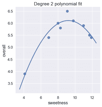 ``` # HIDDEN sns.lmplot(x='sweetness', y='overall', data=ice, fit_reg=False) xs = np.linspace(3.5, 12.5, 1000).reshape(-1, 1) ys = clf.predict(transformer.transform(xs)) plt.plot(xs, ys) plt.title('Degree 2 polynomial fit'); ```  這個模型看起來比我們的線性模型更適合。我們也可以驗證二次多項式擬合的均方成本遠低于線性擬合的成本。 ``` # HIDDEN y = ice['overall'] pred_linear = ( LinearRegression(fit_intercept=False).fit(first_X, y).predict(first_X) ) pred_quad = clf.predict(X) def mse_cost(pred, y): return np.mean((pred - y) ** 2) print(f'MSE cost for linear reg: {mse_cost(pred_linear, y):.3f}') print(f'MSE cost for deg 2 poly reg: {mse_cost(pred_quad, y):.3f}') ``` ``` MSE cost for linear reg: 0.323 MSE cost for deg 2 poly reg: 0.032 ``` ## 增加度數[?](#Increasing-the-Degree) 如前所述，我們可以自由地向數據添加更高階多項式特征。例如，我們可以很容易地創建五次多項式特征： ``` # HIDDEN second_X = PolynomialFeatures(degree=5).fit_transform(ice[['sweetness']]) pd.DataFrame(data=second_X, columns=['bias', 'sweetness', 'sweetness^2', 'sweetness^3', 'sweetness^4', 'sweetness^5']) ``` | | bias | sweetness | sweetness^2 | 甜度^3 | 甜度^4 | 甜度^5 | | --- | --- | --- | --- | --- | --- | --- | | 0 | 1.0 | 4.1 | 16.81 | 六十八點九二一 | 282.5761 個 | 1158.56201 年 | | --- | --- | --- | --- | --- | --- | --- | | 1 | 1.0 | 6.9 | 47.61 | 328.509 年 | 2266.7121 個 | 15640.31349 年 | | --- | --- | --- | --- | --- | --- | --- | | 2 | 1.0 | 8.3 | 68.89 | 571.787 美元 | 4745.8321 個 | 39390.40643 個 | | --- | --- | --- | --- | --- | --- | --- | | ... | ... | ... | ... | ... | ... | ... | | --- | --- | --- | --- | --- | --- | --- | | 6 | 1.0 | 11.0 | 121.00 | 1331.000 個 | 14641.0000 元 | 161051.00000 美元 | | --- | --- | --- | --- | --- | --- | --- | | 7 | 1.0 | 11.7 | 136.89 | 1601.613 年 | 18738.8721 年 | 219244.80357 號 | | --- | --- | --- | --- | --- | --- | --- | | 8 | 1.0 | 11.9 | 141.61 | 1685.159 年 | 20053.3921 年 | 238635.36599 個 | | --- | --- | --- | --- | --- | --- | --- | 9 行×6 列 利用這些特征擬合線性模型，得到五次多項式回歸。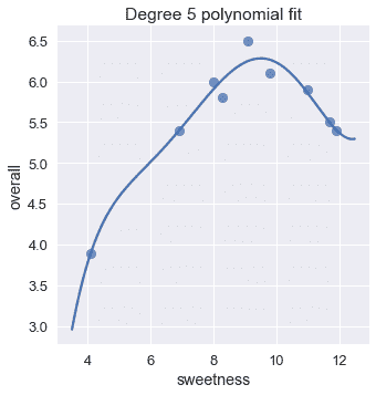 ``` # HIDDEN trans_five = PolynomialFeatures(degree=5) X_five = trans_five.fit_transform(ice[['sweetness']]) clf_five = LinearRegression(fit_intercept=False).fit(X_five, y) sns.lmplot(x='sweetness', y='overall', data=ice, fit_reg=False) xs = np.linspace(3.5, 12.5, 1000).reshape(-1, 1) ys = clf_five.predict(trans_five.transform(xs)) plt.plot(xs, ys) plt.title('Degree 5 polynomial fit'); ```  該圖表明，一個五次多項式和一個二次多項式似乎能大致擬合數據。事實上，五次多項式的均方成本幾乎是二次多項式成本的一半。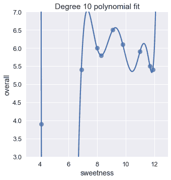 ``` pred_five = clf_five.predict(X_five) print(f'MSE cost for linear reg: {mse_cost(pred_linear, y):.3f}') print(f'MSE cost for deg 2 poly reg: {mse_cost(pred_quad, y):.3f}') print(f'MSE cost for deg 5 poly reg: {mse_cost(pred_five, y):.3f}') ``` ``` MSE cost for linear reg: 0.323 MSE cost for deg 2 poly reg: 0.032 MSE cost for deg 5 poly reg: 0.017 ``` 這表明，我們可能會做得更好，提高程度甚至更多。為什么不是 10 次多項式？ ``` # HIDDEN trans_ten = PolynomialFeatures(degree=10) X_ten = trans_ten.fit_transform(ice[['sweetness']]) clf_ten = LinearRegression(fit_intercept=False).fit(X_ten, y) sns.lmplot(x='sweetness', y='overall', data=ice, fit_reg=False) xs = np.linspace(3.5, 12.5, 1000).reshape(-1, 1) ys = clf_ten.predict(trans_ten.transform(xs)) plt.plot(xs, ys) plt.title('Degree 10 polynomial fit') plt.ylim(3, 7); ```  下面是迄今為止我們所看到的回歸模型的均方成本： ``` # HIDDEN pred_ten = clf_ten.predict(X_ten) print(f'MSE cost for linear reg: {mse_cost(pred_linear, y):.3f}') print(f'MSE cost for deg 2 poly reg: {mse_cost(pred_quad, y):.3f}') print(f'MSE cost for deg 5 poly reg: {mse_cost(pred_five, y):.3f}') print(f'MSE cost for deg 10 poly reg: {mse_cost(pred_ten, y):.3f}') ``` ``` MSE cost for linear reg: 0.323 MSE cost for deg 2 poly reg: 0.032 MSE cost for deg 5 poly reg: 0.017 MSE cost for deg 10 poly reg: 0.000 ``` 10 次多項式的代價為零！如果我們仔細觀察這個圖，這是有意義的；十次多項式設法通過數據中每個點的精確位置。 然而，你應該對使用 10 次多項式來預測冰淇淋評級感到猶豫。直觀地說，10 次多項式似乎與我們的特定數據集太接近了。如果我們取另一組數據，并將它們繪制在上面的散點圖上，我們可以期望它們接近我們的原始數據集。然而，當我們這樣做時，10 次多項式突然看起來不太合適，而 2 次多項式看起來仍然合理。 ``` # HIDDEN # sns.lmplot(x='sweetness', y='overall', data=ice, fit_reg=False) np.random.seed(1) x_devs = np.random.normal(scale=0.4, size=len(ice)) y_devs = np.random.normal(scale=0.4, size=len(ice)) plt.figure(figsize=(10, 5)) # Degree 10 plt.subplot(121) ys = clf_ten.predict(trans_ten.transform(xs)) plt.plot(xs, ys) plt.scatter(ice['sweetness'] + x_devs, ice['overall'] + y_devs, c='g') plt.title('Degree 10 poly, second set of data') plt.ylim(3, 7); plt.subplot(122) ys = clf.predict(transformer.transform(xs)) plt.plot(xs, ys) plt.scatter(ice['sweetness'] + x_devs, ice['overall'] + y_devs, c='g') plt.title('Degree 2 poly, second set of data') plt.ylim(3, 7); ```  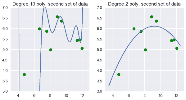我們可以看到，在這種情況下，二次多項式的特征比無變換和十次多項式的特征都更好。 這就提出了一個自然的問題：一般來說，我們如何確定要擬合的多項式的度數？盡管我們試圖使用訓練數據集上的成本來選擇最佳多項式，但我們已經看到使用此成本可以選擇過于復雜的模型。相反，我們希望根據不用于擬合參數的數據來評估模型。 ## 摘要[?](#Summary) 在本節中，我們將介紹另一種特征工程技術：將多項式特征添加到數據中以執行多項式回歸。與一種熱編碼一樣，添加多項式特性允許我們在更多類型的數據上有效地使用線性回歸模型。 我們還遇到了特征工程的一個基本問題。向數據中添加許多特性可以使模型在其原始數據集上降低成本，但通常會導致新數據集上的模型不太精確。