# 交叉驗證 > 原文：[https://www.textbook.ds100.org/ch/15/bias_cv.html](https://www.textbook.ds100.org/ch/15/bias_cv.html) ``` # HIDDEN # Clear previously defined variables %reset -f # Set directory for data loading to work properly import os os.chdir(os.path.expanduser('~/notebooks/15')) ``` ``` # HIDDEN import warnings # Ignore numpy dtype warnings. These warnings are caused by an interaction # between numpy and Cython and can be safely ignored. # Reference: https://stackoverflow.com/a/40846742 warnings.filterwarnings("ignore", message="numpy.dtype size changed") warnings.filterwarnings("ignore", message="numpy.ufunc size changed") import numpy as np import matplotlib.pyplot as plt import pandas as pd import seaborn as sns %matplotlib inline import ipywidgets as widgets from ipywidgets import interact, interactive, fixed, interact_manual import nbinteract as nbi sns.set() sns.set_context('talk') np.set_printoptions(threshold=20, precision=2, suppress=True) pd.options.display.max_rows = 7 pd.options.display.max_columns = 8 pd.set_option('precision', 2) # This option stops scientific notation for pandas # pd.set_option('display.float_format', '{:.2f}'.format) ``` ``` # HIDDEN def df_interact(df, nrows=7, ncols=7): ''' Outputs sliders that show rows and columns of df ''' def peek(row=0, col=0): return df.iloc[row:row + nrows, col:col + ncols] if len(df.columns) <= ncols: interact(peek, row=(0, len(df) - nrows, nrows), col=fixed(0)) else: interact(peek, row=(0, len(df) - nrows, nrows), col=(0, len(df.columns) - ncols)) print('({} rows, {} columns) total'.format(df.shape[0], df.shape[1])) ``` 在前一節中，我們觀察到，我們需要一種更精確的方法來模擬測試誤差來管理偏差方差權衡。重申一下，由于我們正在將我們的模型擬合到訓練集上，因此訓練誤差非常低。我們需要在不使用測試集的情況下選擇一個模型，因此我們再次將我們的培訓集分割成一個驗證集。交叉驗證提供了一種方法，通過將用于培訓的數據與用于模型選擇和最終精度的數據分離，使用單個觀測數據集估計模型誤差。 ## 列車驗證試驗拆分 實現這一點的一種方法是將原始數據集拆分為三個不相交的子集： * 訓練集：用于擬合模型的數據。 * 驗證集：用于選擇功能的數據。 * 測試集：用于報告模型最終精度的數據。 拆分后，我們根據以下步驟選擇一組特征和一個模型： 1. 對于每個潛在的功能集，使用訓練集擬合模型。模型在訓練集上的錯誤是它的 _ 訓練錯誤 _。 2. 檢查驗證集上每個模型的錯誤：其 _ 驗證錯誤 _。選擇實現最低驗證錯誤的模型。這是功能和模型的最終選擇。 3. 計算測試集上最終模型的 _ 測試誤差 _，誤差。這是模型的最終報告精度。我們禁止調整特性或模型以減少測試錯誤；這樣做可以有效地將測試集轉換為驗證集。相反，我們必須在對特性或模型進行進一步更改之后收集一個新的測試集。 這個過程允許我們比單獨使用訓練錯誤更準確地確定要使用的模型。通過交叉驗證，我們可以在不適合的數據上測試我們的模型，在不使用測試集的情況下模擬測試錯誤。這讓我們了解了我們的模型是如何對看不見的數據執行的。 **列車驗證試驗段尺寸** 列車驗證測試拆分通常使用 70%的數據作為訓練集，15%作為驗證集，其余 15%作為測試集。增加訓練集的大小有助于模型的準確性，但會導致驗證和測試錯誤的更多變化。這是因為較小的驗證集和測試集對樣本數據的代表性較小。 ## 訓練錯誤和測試錯誤 如果一個模型不能推廣到人口中看不見的數據，那么它對我們幾乎沒有用處。由于我們不使用測試集來訓練模型或選擇特性，因此測試錯誤可以最準確地表示模型在新數據上的性能。 一般來說，訓練誤差會隨著模型的復雜度的增加而減小，因為模型具有附加的特性或更復雜的預測機制。另一方面，測試誤差降低到一定程度的復雜性，然后隨著模型與訓練集的過度匹配而再次增加。這是由于這樣一個事實：首先，偏差的減少大于方差的增加。最終，方差的增加超過了偏差的減少。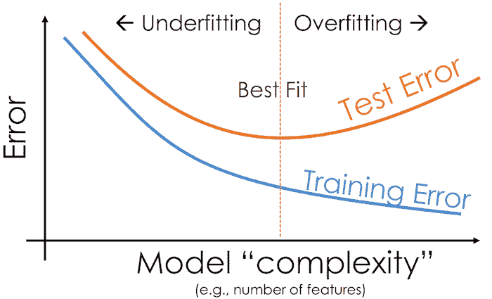 ## K-折疊交叉驗證 **列車驗證測試拆分**方法是通過驗證集模擬試驗誤差的一種好方法。但是，進行三個分割會導致訓練數據太少。此外，使用這種方法，驗證錯誤可能會傾向于高方差，因為對錯誤的評估很大程度上取決于培訓和驗證集中的結束點。 為了解決這個問題，我們可以在同一個數據集中多次運行列車驗證拆分。數據集分為 _k_ 等大小的子集（_$k$folds_），列車驗證拆分重復 _k_ 次。每次使用一個 _k_ 折疊作為驗證集，剩余的 _k-1_ 折疊用作培訓集。我們將模型的最終驗證錯誤報告為每個試驗$k$驗證錯誤的平均值。此方法稱為**K-折疊交叉驗證**。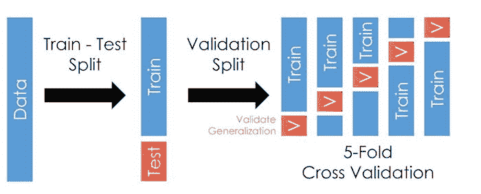 下圖說明了使用五個折疊時的技術：  該方法的最大優點是，每個數據點僅用于一次驗證和訓練 _K-1_ 次。通常，使用介于 5 到 10 之間的 _k_，但 _k_ 仍是未固定的參數。當 _k_ 很小時，誤差估計具有較低的方差（許多驗證點），但具有較高的偏差（較少的訓練點）。反之，當 _k_ 較大時，誤差估計的偏差較小，但方差較大。 $K$折疊交叉驗證比火車驗證拆分需要更多的計算時間，因為我們通常必須為每個折疊從頭重新安裝每個模型。但是，它通過對每個模型的多個錯誤進行平均來計算更精確的驗證錯誤。 `scikit-learn`庫提供了一個方便的[`sklearn.model_selection.KFold`](http://scikit-learn.org/stable/modules/generated/sklearn.model_selection.KFold.html)類來實現$k$的交叉驗證。 ## 偏差方差權衡 交叉驗證有助于我們更準確地管理偏差-方差權衡。直觀地說，驗證錯誤通過在不用于培訓的數據集上檢查模型的性能來估計測試錯誤；這允許我們同時估計模型偏差和模型方差。k 倍交叉驗證還包括這樣一個事實：測試集中的噪聲只影響偏差方差分解中的噪聲項，而訓練集中的噪聲同時影響偏差和模型方差。要選擇要使用的最終模型，我們選擇驗證錯誤最小的模型。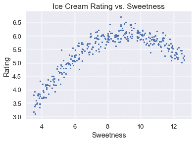 ## 示例：冰淇淋評級的型號選擇[?](#Example:-Model-Selection-for-Ice-Cream-Ratings) 我們將使用完整的模型選擇過程，包括交叉驗證，來選擇一個預測冰淇淋甜度等級的模型。完整的冰淇淋數據集和整體評分與冰淇淋甜度的散點圖如下所示。 ``` # HIDDEN ice = pd.read_csv('icecream.csv') transformer = PolynomialFeatures(degree=2) X = transformer.fit_transform(ice[['sweetness']]) clf = LinearRegression(fit_intercept=False).fit(X, ice[['overall']]) xs = np.linspace(3.5, 12.5, 300).reshape(-1, 1) rating_pred = clf.predict(transformer.transform(xs)) temp = pd.DataFrame(xs, columns = ['sweetness']) temp['overall'] = rating_pred np.random.seed(42) x_devs = np.random.normal(scale=0.2, size=len(temp)) y_devs = np.random.normal(scale=0.2, size=len(temp)) temp['sweetness'] = np.round(temp['sweetness'] + x_devs, decimals=2) temp['overall'] = np.round(temp['overall'] + y_devs, decimals=2) ice = pd.concat([temp, ice]) ``` ``` ice ``` | | 甜度 | 總體的 | | --- | --- | --- | | 零 | 3.60 條 | 三點零九 | | --- | --- | --- | | 1 個 | 3.50 美元 | 三點一七 | | --- | --- | --- | | 二 | 三點六九 | 三點四六 | | --- | --- | --- | | …… | …… | ... | | --- | --- | --- | | 六 | 十一 | 五點九零 | | --- | --- | --- | | 七 | 十一點七零 | 5.50 美元 | | --- | --- | --- | | 8 個 | 十一點九零 | 五點四零 | | --- | --- | --- | 309 行×2 列 ``` # HIDDEN plt.scatter(ice['sweetness'], ice['overall'], s=10) plt.title('Ice Cream Rating vs. 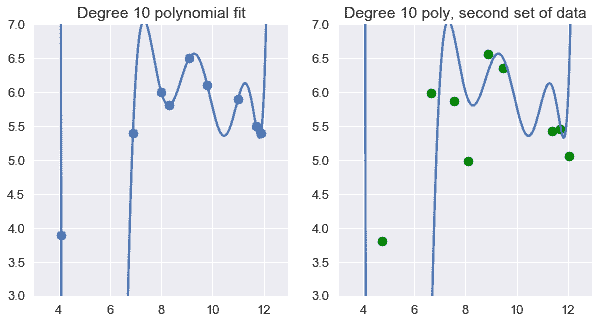Sweetness') plt.xlabel('Sweetness') plt.ylabel('Rating'); ```  在數據集中的 9 個隨機點上使用 10 次多項式特征，可以得到這些數據點的精確模型。不幸的是，這個模型不能概括為以前從總體中看不到的數據。 ``` # HIDDEN from sklearn.preprocessing import PolynomialFeatures from sklearn.linear_model import LinearRegression ice2 = pd.read_csv('icecream.csv') trans_ten = PolynomialFeatures(degree=10) X_ten = trans_ten.fit_transform(ice2[['sweetness']]) y = ice2['overall'] clf_ten = LinearRegression(fit_intercept=False).fit(X_ten, y) ``` ``` # HIDDEN np.random.seed(1) x_devs = np.random.normal(scale=0.4, size=len(ice2)) y_devs = np.random.normal(scale=0.4, size=len(ice2)) plt.figure(figsize=(10, 5)) plt.subplot(121) plt.scatter(ice2['sweetness'], ice2['overall']) xs = np.linspace(3.5, 12.5, 1000).reshape(-1, 1) ys = clf_ten.predict(trans_ten.transform(xs)) plt.plot(xs, ys) plt.title('Degree 10 polynomial fit') plt.ylim(3, 7); plt.subplot(122) ys = clf_ten.predict(trans_ten.transform(xs)) plt.plot(xs, ys) plt.scatter(ice2['sweetness'] + x_devs, ice2['overall'] + y_devs, c='g') plt.title('Degree 10 poly, second set of data') plt.ylim(3, 7); ```  代替上述方法，我們首先使用`scikit-learn`'s[`sklearn.model_selection.train_test_split`](http://scikit-learn.org/stable/modules/generated/sklearn.model_selection.train_test_split.html)方法將數據劃分為培訓、驗證和測試數據集，以執行 70/30%的列車測試分割。 ``` from sklearn.model_selection import train_test_split test_size = 92 X_train, X_test, y_train, y_test = train_test_split( ice[['sweetness']], ice['overall'], test_size=test_size, random_state=0) print(f' Training set size: {len(X_train)}') print(f' Test set size: {len(X_test)}') ``` ``` Training set size: 217 Test set size: 92 ``` 我們現在使用訓練集擬合多項式回歸模型，每個多項式階數從 1 到 10 為一個。 ``` from sklearn.linear_model import LinearRegression from sklearn.preprocessing import PolynomialFeatures # First, we add polynomial features to X_train transformers = [PolynomialFeatures(degree=deg) for deg in range(1, 11)] X_train_polys = [transformer.fit_transform(X_train) for transformer in transformers] # Display the X_train with degree 5 polynomial features X_train_polys[4] ``` ``` array([[ 1\. , 8.8 , 77.44, 681.47, 5996.95, 52773.19], [ 1\. , 10.74, 115.35, 1238.83, 13305.07, 142896.44], [ 1\. , 9.98, 99.6 , 994.01, 9920.24, 99003.99], ..., [ 1\. , 6.79, 46.1 , 313.05, 2125.59, 14432.74], [ 1\. , 5.13, 26.32, 135.01, 692.58, 3552.93], [ 1\. , 8.66, 75\. , 649.46, 5624.34, 48706.78]]) ``` 然后我們將對 10 個特征數據集執行 5 倍交叉驗證。為此，我們將定義一個函數： 1. 使用[`KFold.split`](http://scikit-learn.org/stable/modules/generated/sklearn.model_selection.KFold.html)函數獲取訓練數據的 5 個拆分。請注意，`split`返回該拆分數據的索引。 2. 對于每個拆分，根據拆分索引和特征選擇行和列。 3. 在訓練分割上擬合線性模型。 4. 計算驗證拆分的均方誤差。 5. 返回所有交叉驗證拆分的平均錯誤。 ``` from sklearn.model_selection import KFold def mse_cost(y_pred, y_actual): return np.mean((y_pred - y_actual) ** 2) def compute_CV_error(model, X_train, Y_train): kf = KFold(n_splits=5) validation_errors = [] for train_idx, valid_idx in kf.split(X_train): # split the data split_X_train, split_X_valid = X_train[train_idx], X_train[valid_idx] split_Y_train, split_Y_valid = Y_train.iloc[train_idx], Y_train.iloc[valid_idx] # Fit the model on the training split model.fit(split_X_train,split_Y_train) # Compute the RMSE on the validation split error = mse_cost(split_Y_valid,model.predict(split_X_valid)) validation_errors.append(error) #average validation errors return np.mean(validation_errors) ``` ``` # We train a linear regression classifier for each featurized dataset and perform cross-validation # We set fit_intercept=False for our linear regression classifier since # the PolynomialFeatures transformer adds the bias column for us. cross_validation_errors = [compute_CV_error(LinearRegression(fit_intercept=False), X_train_poly, y_train) for X_train_poly in X_train_polys] ``` ``` # HIDDEN cv_df = pd.DataFrame({'Validation Error': cross_validation_errors}, index=range(1, 11)) cv_df.index.name = 'Degree' pd.options.display.max_rows = 20 display(cv_df) pd.options.display.max_rows = 7 ``` | | 驗證錯誤 | | --- | --- | | 度 | | | --- | --- | | 1 | 0.324820 個 | | --- | --- | | 2 | 0.045060 | | --- | --- | | 三 | 0.045418 | | --- | --- | | 四 | 0.045282 個 | | --- | --- | | 5 個 | 0.046272 | | --- | --- | | 6 | 0.046715 | | --- | --- | | 7 | 0.047140 | | --- | --- | | 8 | 0.047540 | | --- | --- | | 九 | 0.048055 | | --- | --- | | 10 個 | 0.047805 | | --- | --- | 我們可以看到，當我們使用更高階多項式特征時，驗證誤差會減少和增加。 ``` # HIDDEN plt.figure(figsize=(10, 5)) plt.subplot(121) plt.plot(cv_df.index, cv_df['Validation Error']) plt.scatter(cv_df.index, cv_df['Validation Error']) plt.title('Validation Error vs. 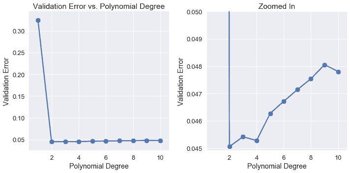Polynomial Degree') plt.xlabel('Polynomial Degree') plt.ylabel('Validation Error'); plt.subplot(122) plt.plot(cv_df.index, cv_df['Validation Error']) plt.scatter(cv_df.index, cv_df['Validation Error']) plt.ylim(0.044925, 0.05) plt.title('Zoomed In') plt.xlabel('Polynomial Degree') plt.ylabel('Validation Error') plt.tight_layout(); ```  檢驗驗證誤差表明，最精確的模型只使用二次多項式特征。因此，我們選擇二次多項式模型作為最終模型，并將其一次擬合到所有訓練數據上。然后，我們在測試集中計算它的錯誤。 ``` best_trans = transformers[1] best_model = LinearRegression(fit_intercept=False).fit(X_train_polys[1], y_train) training_error = mse_cost(best_model.predict(X_train_polys[1]), y_train) validation_error = cross_validation_errors[1] test_error = mse_cost(best_model.predict(best_trans.transform(X_test)), y_test) print('Degree 2 polynomial') print(f' Training error: {training_error:0.5f}') print(f'Validation error: {validation_error:0.5f}') print(f' Test error: {test_error:0.5f}') ``` ``` Degree 2 polynomial Training error: 0.04409 Validation error: 0.04506 Test error: 0.04698 ``` 為了將來的參考，`scikit-learn`有一個[`cross_val_predict`](http://scikit-learn.org/stable/modules/generated/sklearn.model_selection.cross_val_predict.html)方法來自動執行交叉驗證，所以我們不必自己將數據分解為訓練集和驗證集。 另外，請注意，測試誤差大于驗證誤差，驗證誤差大于訓練誤差。訓練誤差應該是最小的，因為模型適合訓練數據。擬合模型可以最大限度地減少該數據集的均方誤差。驗證誤差和測試誤差通常高于訓練誤差，因為誤差是在模型未看到的未知數據集上計算的。 ## 摘要[?](#Summary) 我們使用廣泛使用的交叉驗證技術來管理偏差-方差權衡。在計算了原始數據集上的列車驗證測試分割后，我們使用以下過程來訓練和選擇模型。 1. 對于每個潛在的功能集，使用訓練集擬合模型。模型在訓練集上的錯誤是它的 _ 訓練錯誤 _。 2. 使用$K$交叉驗證檢查驗證集上每個模型的錯誤：其 _ 驗證錯誤 _。選擇實現最低驗證錯誤的模型。這是功能和模型的最終選擇。 3. 計算測試集上最終模型的 _ 測試誤差 _，誤差。這是模型的最終報告精度。我們禁止調整模型以增加測試錯誤；這樣做可以有效地將測試集轉換為驗證集。相反，我們必須在對模型進行進一步更改之后收集一個新的測試集。