# 使用邏輯回歸 > 原文：[https://www.textbook.ds100.org/ch/17/classification_log_reg.html](https://www.textbook.ds100.org/ch/17/classification_log_reg.html) ``` # HIDDEN # Clear previously defined variables %reset -f # Set directory for data loading to work properly import os os.chdir(os.path.expanduser('~/notebooks/17')) ``` ``` # HIDDEN import warnings # Ignore numpy dtype warnings. These warnings are caused by an interaction # between numpy and Cython and can be safely ignored. # Reference: https://stackoverflow.com/a/40846742 warnings.filterwarnings("ignore", message="numpy.dtype size changed") warnings.filterwarnings("ignore", message="numpy.ufunc size changed") import numpy as np import matplotlib.pyplot as plt import pandas as pd import seaborn as sns %matplotlib inline import ipywidgets as widgets from ipywidgets import interact, interactive, fixed, interact_manual import nbinteract as nbi sns.set() sns.set_context('talk') np.set_printoptions(threshold=20, precision=2, suppress=True) pd.options.display.max_rows = 7 pd.options.display.max_columns = 8 pd.set_option('precision', 2) # This option stops scientific notation for pandas # pd.set_option('display.float_format', '{:.2f}'.format) ``` ``` # HIDDEN def df_interact(df, nrows=7, ncols=7): ''' Outputs sliders that show rows and columns of df ''' def peek(row=0, col=0): return df.iloc[row:row + nrows, col:col + ncols] if len(df.columns) <= ncols: interact(peek, row=(0, len(df) - nrows, nrows), col=fixed(0)) else: interact(peek, row=(0, len(df) - nrows, nrows), col=(0, len(df.columns) - ncols)) print('({} rows, {} columns) total'.format(df.shape[0], df.shape[1])) ``` ``` # HIDDEN from scipy.optimize import minimize as sci_min def minimize(cost_fn, grad_cost_fn, X, y, progress=True): ''' Uses scipy.minimize to minimize cost_fn using a form of gradient descent. ''' theta = np.zeros(X.shape[1]) iters = 0 def objective(theta): return cost_fn(theta, X, y) def gradient(theta): return grad_cost_fn(theta, X, y) def print_theta(theta): nonlocal iters if progress and iters % progress == 0: print(f'theta: {theta} | cost: {cost_fn(theta, X, y):.2f}') iters += 1 print_theta(theta) return sci_min( objective, theta, method='BFGS', jac=gradient, callback=print_theta, tol=1e-7 ).x ``` 我們已經開發了邏輯回歸的所有組件。首先，用于預測概率的邏輯模型： $$ \begin{aligned} f_\hat{\boldsymbol{\theta}} (\textbf{x}) = \sigma(\hat{\boldsymbol{\theta}} \cdot \textbf{x}) \end{aligned} $$ 然后，交叉熵損失函數： $$ \begin{aligned} L(\boldsymbol{\theta}, \textbf{X}, \textbf{y}) = &= \frac{1}{n} \sum_i \left(- y_i \ln \sigma_i - (1 - y_i) \ln (1 - \sigma_i ) \right) \\ \end{aligned} $$ 最后，梯度下降的交叉熵損失的梯度： $$ \begin{aligned} \nabla_{\boldsymbol{\theta}} L(\boldsymbol{\theta}, \textbf{X}, \textbf{y}) &= - \frac{1}{n} \sum_i \left( y_i - \sigma_i \right) \textbf{X}_i \\ \end{aligned} $$ 在上面的表達式中，我們讓$\textbf \x；$表示 p$輸入數據矩陣的$n 乘以 p$輸入值，$\textbf \123\ \，$\textbf \，$\textbf \123\123 123 123 123 123 \ 123 \ \123 \\\\Thet 公司 A 美元。簡而言之，我們定義了$\sigma \boldsymbol \theta（\textbf x u i）=\sigma（\textbf x u i \cdot \hat \boldsymbol \theta）。 ## 勒布朗射門的邏輯回歸 現在讓我們回到本章開頭所面臨的問題：預測勒布朗·詹姆斯將要投哪一球。我們從加載勒布朗在 2017 年 NBA 季后賽中拍攝的照片開始。 ``` lebron = pd.read_csv('lebron.csv') lebron ``` | | 游戲日期 | 分鐘 | 對手 | 動作類型 | 鏡頭類型 | 射擊距離 | 拍攝 | | --- | --- | --- | --- | --- | --- | --- | --- | | 零 | 20170415 年 | 10 個 | 因德 | 駕駛上籃得分 | 2pt 現場目標 | 零 | 0 | | --- | --- | --- | --- | --- | --- | --- | --- | | 1 個 | 20170415 | 11 個 | IND | Driving Layup Shot | 2PT Field Goal | 0 | 1 個 | | --- | --- | --- | --- | --- | --- | --- | --- | | 二 | 20170415 | 十四 | IND | 上籃得分 | 2PT Field Goal | 0 | 1 | | --- | --- | --- | --- | --- | --- | --- | --- | | …… | …… | ... | ... | ... | ... | ... | ... | | --- | --- | --- | --- | --- | --- | --- | --- | | 三百八十一 | 20170612 年 | 46 歲 | GSW | Driving Layup Shot | 2PT Field Goal | 1 | 1 | | --- | --- | --- | --- | --- | --- | --- | --- | | 382 個 | 20170612 | 47 歲 | GSW | 后仰跳投 | 2PT Field Goal | 14 | 0 | | --- | --- | --- | --- | --- | --- | --- | --- | | 三百八十三 | 20170612 | 48 歲 | GSW | Driving Layup Shot | 2PT Field Goal | 二 | 1 | | --- | --- | --- | --- | --- | --- | --- | --- | 384 行×7 列 我們在下面包含了一個小部件，允許您瀏覽整個數據幀。 ``` df_interact(lebron) ``` <button class="js-nbinteract-widget">Loading widgets...</button> ``` (384 rows, 7 columns) total ``` 我們首先只使用拍攝距離來預測拍攝是否進行。`scikit-learn`方便地提供了一個邏輯回歸分類器作為[`sklearn.linear_model.LogisticRegression`](http://scikit-learn.org/stable/modules/generated/sklearn.linear_model.LogisticRegression.html)類。為了使用這個類，我們首先創建數據矩陣`X`和觀察結果向量`y`。 ``` X = lebron[['shot_distance']].as_matrix() y = lebron['shot_made'].as_matrix() print('X:') print(X) print() print('y:') print(y) ``` ``` X: [[ 0] [ 0] [ 0] ... [ 1] [14] [ 2]] y: [0 1 1 ... 1 0 1] ``` 按照慣例，我們將數據分成一個訓練集和一個測試集。 ``` from sklearn.model_selection import train_test_split X_train, X_test, y_train, y_test = train_test_split( X, y, test_size=40, random_state=42 ) print(f'Training set size: {len(y_train)}') print(f'Test set size: {len(y_test)}') ``` ``` Training set size: 344 Test set size: 40 ``` `scikit-learn`使初始化分類器并將其安裝在`X_train`和`y_train`上變得簡單： ``` from sklearn.linear_model import LogisticRegression simple_clf = LogisticRegression() simple_clf.fit(X_train, y_train) ``` ``` LogisticRegression(C=1.0, class_weight=None, dual=False, fit_intercept=True, intercept_scaling=1, max_iter=100, multi_class='ovr', n_jobs=1, penalty='l2', random_state=None, solver='liblinear', tol=0.0001, verbose=0, warm_start=False) ``` 為了可視化分類器的性能，我們繪制了原始點和分類器的預測概率。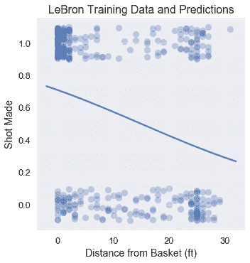 ``` # HIDDEN np.random.seed(42) sns.lmplot(x='shot_distance', y='shot_made', data=lebron, fit_reg=False, ci=False, y_jitter=0.1, scatter_kws={'alpha': 0.3}) xs = np.linspace(-2, 32, 100) ys = simple_clf.predict_proba(xs.reshape(-1, 1))[:, 1] plt.plot(xs, ys) plt.title('LeBron Training Data and Predictions') plt.xlabel('Distance from Basket (ft)') plt.ylabel('Shot Made'); ```  ## 正在評估分類器[?](#Evaluating-the-Classifier) 評估分類器有效性的一種方法是檢查其預測精度：它正確預測的點數比例是多少？ ``` simple_clf.score(X_test, y_test) ``` ``` 0.6 ``` 我們的分類器在測試集上實現了相當低的精度 0.60。如果我們的分類器只是隨機地猜測每個點，那么我們期望精度為 0.50。事實上，如果我們的分類器簡單地預測到 Lebron 的每一次射門都會成功，我們也會得到 0.60 的準確度： ``` # Calculates the accuracy if we always predict 1 np.count_nonzero(y_test == 1) / len(y_test) ``` ``` 0.6 ``` 對于這個分類器，我們只使用了幾個可能的特性中的一個。在多變量線性回歸中，我們可能通過合并更多的特征來實現更精確的分類器。 ## 多變量邏輯回歸 在我們的分類器中合并更多的數字特性就如同從`lebron`數據幀中提取額外的列到`X`矩陣中一樣簡單。另一方面，結合分類特征需要我們應用一個熱編碼。在下面的代碼中，我們使用`minute`、`opponent`、`action_type`和`shot_type`功能增強了分類器，使用`scikit-learn`中的`DictVectorizer`類對分類變量應用一個熱編碼。 ``` from sklearn.feature_extraction import DictVectorizer columns = ['shot_distance', 'minute', 'action_type', 'shot_type', 'opponent'] rows = lebron[columns].to_dict(orient='row') onehot = DictVectorizer(sparse=False).fit(rows) X = onehot.transform(rows) y = lebron['shot_made'].as_matrix() X.shape ``` ``` (384, 42) ``` 我們將再次將數據分為訓練集和測試集： ``` X_train, X_test, y_train, y_test = train_test_split( X, y, test_size=40, random_state=42 ) print(f'Training set size: {len(y_train)}') print(f'Test set size: {len(y_test)}') ``` ``` Training set size: 344 Test set size: 40 ``` 最后，我們再次調整模型并檢查其準確性： ``` clf = LogisticRegression() clf.fit(X_train, y_train) print(f'Test set accuracy: {clf.score(X_test, y_test)}') ``` ``` Test set accuracy: 0.725 ``` 這個分類器比只考慮射擊距離的分類器精確 12%左右。在第 17.7 節中，我們探討了用于評估分類器性能的其他指標。 ## 摘要[?](#Summary) 我們開發了使用邏輯回歸進行分類所需的數學和計算機制。邏輯回歸因其預測簡單有效而得到廣泛應用。