# 最小二乘-幾何透視 > 原文：[https://www.textbook.ds100.org/ch/13/linear_projection.html](https://www.textbook.ds100.org/ch/13/linear_projection.html) ``` # HIDDEN # Clear previously defined variables %reset -f # Set directory for data loading to work properly import os os.chdir(os.path.expanduser('~/notebooks/13')) ``` ``` # HIDDEN import warnings # Ignore numpy dtype warnings. These warnings are caused by an interaction # between numpy and Cython and can be safely ignored. # Reference: https://stackoverflow.com/a/40846742 warnings.filterwarnings("ignore", message="numpy.dtype size changed") warnings.filterwarnings("ignore", message="numpy.ufunc size changed") import numpy as np import matplotlib.pyplot as plt import pandas as pd import seaborn as sns %matplotlib inline import ipywidgets as widgets from ipywidgets import interact, interactive, fixed, interact_manual import nbinteract as nbi sns.set() sns.set_context('talk') np.set_printoptions(threshold=20, precision=2, suppress=True) pd.options.display.max_rows = 7 pd.options.display.max_columns = 8 pd.set_option('precision', 2) # This option stops scientific notation for pandas # pd.set_option('display.float_format', '{:.2f}'.format) ``` 通過對線性模型的損失函數進行梯度下降優化，得到了線性模型的最優系數。我們還提到，最小二乘線性回歸可以用解析法求解。雖然梯度下降是可行的，但這種幾何視角將提供對線性回歸的更深入的理解。 附錄中包括矢量空間審查。我們假設熟悉向量算法、1 向量、向量集合的跨度和投影。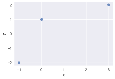 ## 案例研究 我們的任務是為數據找到一個好的線性模型： | X | 是 | | --- | --- | | 三 | 二 | | 零 | 1 個 | | - 1 | - 2 | ``` # HIDDEN data = pd.DataFrame( [ [3,2], [0,1], [-1,-2] ], columns=['x', 'y'] ) sns.regplot(x='x', y='y', data=data, ci=None, fit_reg=False); ```  假設最佳模型是誤差最小的模型，最小二乘誤差是可接受的度量。 ### 最小二乘法：常數模型[?](#Least-Squares:-Constant-Model) 就像我們對 Tips 數據集所做的那樣，讓我們從常量模型開始：這個模型只預測一個數字。 $$ \theta = C$$ 因此，我們只處理$Y$值。 | y | | --- | | 2 | | 1 | | -2 | 我們的目標是找到導致平方損失最小的那一行的$\theta$ $$ L(\theta, \textbf{y}) = \sum_{i = 1}^{n}(y_i - \theta)^2\\ $$ 回想一下，對于常量模型，MSE 的最小化$\theta$是$\bar \textbf y$，是$\textbf y 值的平均值。微積分推導可在“建模和估計”一章的“損失函數”一課中找到。關于線性代數推導，請參閱附錄中的向量空間回顧。 注意我們的損失函數是平方和。向量的 _l2_-范數也是平方和，但具有平方根： $$\Vert \textbf{v} \Vert = \sqrt{v_1^2 + v_2^2 + \dots + v_n^2}$$ 如果我們讓$y_i-\theta=v_i$： $$ \begin{aligned} L(\theta, \textbf{y}) &= v_1^2 + v_2^2 + \dots + v_n^2 \\ &= \Vert \textbf{v} \Vert^2 \end{aligned} $$ 這意味著我們的損失可以表示為一些向量的 _l2_-范數$\textbf v，$的平方。我們可以用[1，n]$將所有 i 的$v_i$表示為$y_i-\theta\quad\，這樣用笛卡爾符號表示， $$ \begin{aligned} \textbf{v} \quad &= \quad \begin{bmatrix} y_1 - \theta \\ y_2 - \theta \\ \vdots \\ y_n - \theta \end{bmatrix} \\ &= \quad \begin{bmatrix} y_1 \\ y_2 \\ \vdots \\ y_n \end{bmatrix} \quad - \quad \begin{bmatrix} \theta \\ \theta \\ \vdots \\ \theta \end{bmatrix} \\ &= \quad \begin{bmatrix} y_1 \\ y_2 \\ \vdots \\ y_n \end{bmatrix} \quad - \quad \theta \begin{bmatrix} 1 \\ 1 \\ \vdots \\ 1 \end{bmatrix} \end{aligned} $$ 因此，我們的損失函數可以寫為： $$ \begin{aligned} L(\theta, \textbf{y}) \quad &= \quad \left \Vert \qquad \begin{bmatrix} y_1 \\ y_2 \\ \vdots \\ y_n \end{bmatrix} \quad - \quad \theta \begin{bmatrix} 1 \\ 1 \\ \vdots \\ 1 \end{bmatrix} \qquad \right \Vert ^2 \\ \quad &= \quad \left \Vert \qquad \textbf{y} \quad - \quad \hat{\textbf{y}} \qquad \right \Vert ^2 \\ \end{aligned} $$ 表達式$\theta\begin bmatrix 1\\1\\vdots\\1\end bmatrix$是$\textbf 1 矢量列的標量倍數，是我們預測的結果，表示為$\hat \textbf y。 這就為我們提供了一個新的視角來理解最小化最小二乘誤差意味著什么。 $\textbf y 和$\textbf 1 是固定的，但$\theta$可以具有任何值，因此$\hat \textbf y 可以是$\textbf 1 的任何標量倍數。我們希望找到$\theta$以便$\theta\textbf 1$盡可能接近$\textbf y$。我們使用$\hat \theta$來表示這個最適合的$\theta$。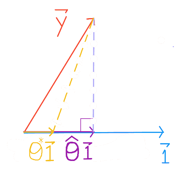  將$\textbf y$投影到$\textbf 1$上，保證是最接近的矢量（參見附錄中的“矢量空間回顧”）。 ### 最小二乘法：簡單線性模型 現在，讓我們看看簡單的線性回歸模型。這與常數模型推導非常相似，但是要注意這些差異，并考慮如何推廣到多重線性回歸。 簡單的線性模型是： $$ \begin{aligned} f_\boldsymbol\theta (x_i) &= \theta_0 + \theta_1 x_i \\ \end{aligned} $$ 我們的目標是找到導致最小平方誤差行的$\BoldSymbol\Theta$： $$ \begin{aligned} L(\boldsymbol\theta, \textbf{x}, \textbf{y}) &= \sum_{i = 1}^{n}(y_i - f_\boldsymbol\theta (x_i))^2\\ &= \sum_{i = 1}^{n}(y_i - \theta_0 - \theta_1 x_i)^2\\ &= \sum_{i = 1}^{n}(y_i - \begin{bmatrix} 1 & x_i \end{bmatrix} \begin{bmatrix} \theta_0 \\ \theta_1 \end{bmatrix} ) ^2 \end{aligned} $$ 為了幫助我們將損失求和轉換為矩陣形式，讓我們用$n=3$展開損失。 $$ \begin{aligned} L(\boldsymbol{\theta}, \textbf{x}, \textbf{y}) &= (y_1 - \begin{bmatrix} 1 & x_1 \end{bmatrix} \begin{bmatrix} \theta_0 \\ \theta_1 \end{bmatrix})^2 \\ &+ (y_2 - \begin{bmatrix} 1 & x_2 \end{bmatrix} \begin{bmatrix} \theta_0 \\ \theta_1 \end{bmatrix})^2 \\ &+ (y_3 - \begin{bmatrix} 1 & x_3 \end{bmatrix} \begin{bmatrix} \theta_0 \\ \theta_1 \end{bmatrix})^2 \\ \end{aligned} $$ 同樣，我們的損失函數是平方和，向量的 _l2_-范數是平方和的平方根： $$\Vert \textbf{v} \Vert = \sqrt{v_1^2 + v_2^2 + \dots + v_n^2}$$ 如果我們讓$y_i-\ begin bmatrix 1&x_u i \ end bmatrix \ begin bmatrix \ theta 0 \ theta end bmatrix=v i$： $$ \begin{aligned} L(\boldsymbol{\theta}, \textbf{x}, \textbf{y}) &= v_1^2 + v_2^2 + \dots + v_n^2 \\ &= \Vert \textbf{v} \Vert^2 \end{aligned} $$ 和以前一樣，我們的損失可以表示為一些向量的 _l2_-范數$\textbf v$，平方。對于[1,3]中所有 i 的組件$v_i=y_i-\ begin bmatrix 1&x_i \ end bmatrix begin bmatrix \ theta \ theta end bmatrix quad \ $$ \begin{aligned} L(\boldsymbol{\theta}, \textbf{x}, \textbf{y}) &= \left \Vert \qquad \begin{bmatrix} y_1 \\ y_2 \\ y_3 \end{bmatrix} \quad - \quad \begin{bmatrix} 1 & x_1 \\ 1 & x_2 \\ 1 & x_3 \end{bmatrix} \begin{bmatrix} \theta_0 \\ \theta_1 \end{bmatrix} \qquad \right \Vert ^2 \\ &= \left \Vert \qquad \textbf{y} \quad - \quad \textbf{X} \begin{bmatrix} \theta_0 \\ \theta_1 \end{bmatrix} \qquad \right \Vert ^2 \\ &= \left \Vert \qquad \textbf{y} \quad - \quad f_\boldsymbol\theta(\textbf{x}) \qquad \right \Vert ^2 \\ &= \left \Vert \qquad \textbf{y} \quad - \quad \hat{\textbf{y}} \qquad \right \Vert ^2 \\ \end{aligned} $$ 矩陣乘法$\ Begin BMatrix 1&x U 1 \ \\1&x U 2 \ \\1&x U 3 \ \端；BMatrix BMatrix \ Theta \ \ \\Theta U 1 \ \ \ \ \端；BMatrix；$是$\textbf x；$列的線性組合：每一個\\theta _i$只有一次乘一列的$\textbf x 123; x；$X；$的一列的-這汗 CTIVE 向我們展示了$F_u \boldSymbol\theta$是我們數據特征的線性組合。 $\textbf x 和$\textbf y 是固定的，但是$\theta 0$和$\theta 1$可以接受任何值，因此$\that \textbf y 可以接受$\textbf x 列的任意無限線性組合。為了獲得最小的損失，我們要選擇$\BoldSymbol\Theta$使$\Hat \textbf y 美元盡可能接近$\textbf y 美元，表示為$\Hat \BoldSymbol\Theta 美元。 ## 幾何直覺 現在，讓我們發展一種直覺，來解釋為什么$\hat \textbf y$僅限于$\textbf x 列的線性組合。雖然任意向量集的跨度包含無限多的線性組合，但無窮并不意味著任何線性組合都受到基向量的限制。 作為提醒，這里是我們的損失函數和散點圖： $$L(\boldsymbol{\theta}, \textbf{x}, \textbf{y}) \quad = \quad \left \Vert \quad \textbf{y} \quad - \quad \textbf{X} \boldsymbol\theta \quad \right \Vert ^2$$ ``` # HIDDEN sns.regplot(x='x', y='y', data=data, ci=None, fit_reg=False); ```  通過查看我們的散點圖，我們發現沒有一條線能夠完美地匹配我們的點，因此我們無法實現 0 損失。因此，我們知道$\textbf y 不在由$\textbf x 和$\textbf 1 所跨越的平面內，下面用一個平行四邊形表示。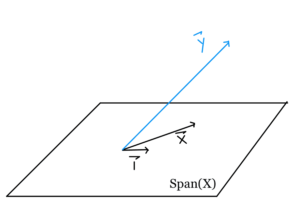  因為我們的損失是基于距離的，所以我們可以看到，為了盡量減少$L（\boldsymbol\theta、\textbf x、\textbf y）=\left\vert\textbf-\textbf x \boldsymbol\theta\right\vert^2$，我們希望$\textbf x \boldsymbol\theta$接近$textbf y。 從數學上來說，我們正在尋找$\textbf y 到由$\textbf x 列所跨越的向量空間的投影，因為任何向量的投影都是$SPAN（\textbf x）$中最接近該向量的點。因此，選擇$\BoldSymbol\Theta$使$\Hat \textbf y=\textbf x \BoldSymbol\Theta=$Proj$SPAN（\textbf x）$$\textbf y 是最佳解決方案。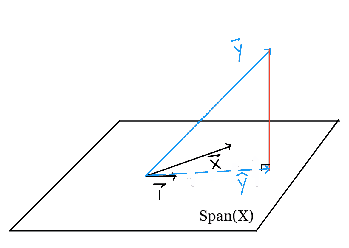 要了解原因，請考慮向量空間上的其他點（紫色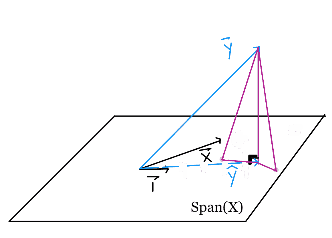）。 根據畢達哥拉斯定理，平面上的任何其他點都離$\textbf y 遠于$\hat \textbf y is。與$\hat \textbf y$對應的垂線長度表示最小平方誤差。 ## 線性代數 因為我們已經學習了很多線性代數概念，剩下的就是解出$\hat \boldSymbol\theta$得到我們想要的$\hat \textbf y$。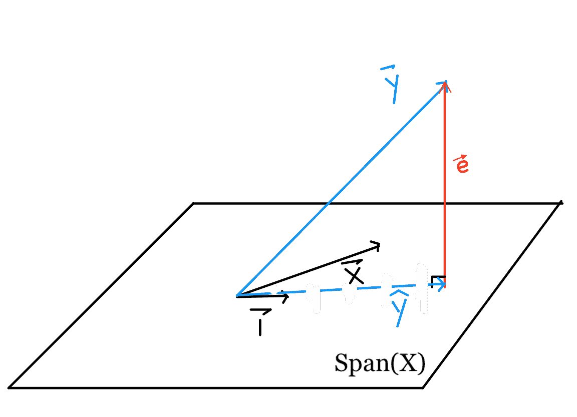 需要注意的幾點：  * $\hat \textbf y+\textbf e=\textbf y$ * $\textbf e 與$\textbf x 和$\textbf 1 垂直$ * $\hat \textbf y=\textbf x \hat \boldsymbol\theta$是最接近\textbf y$的向量空間，該向量空間由$\textbf x 和$\textbf 1 所跨越。$ 因此，我們得出如下方程： $$\textbf{X} \hat{\boldsymbol\theta} + \textbf{e} = \textbf{y}$$ 左乘兩邊的$\textbf x ^t$： $$\textbf{X}^T \textbf{X} \hat{\boldsymbol\theta} + \textbf{X}^T \textbf{e} = \textbf{X}^T \textbf{y}$$ 因為$\textbf e$垂直于$\textbf x$，$\textbf x ^t\textbf e$的列向量。因此，我們得出了正態方程： $$\textbf{X}^T \textbf{X} \hat{\boldsymbol\theta} = \textbf{X}^T \textbf{y}$$ 從這里，我們可以很容易地解出$\Hat \BoldSymbol\Theta$乘以兩邊的$（\textbf x ^t\textbf x）^-1$： $$\hat{\boldsymbol\theta} = (\textbf{X}^T \textbf{X})^{-1} \textbf{X}^T \textbf{y}$$ 注：我們可以通過向量微積分的最小化得到同樣的解，但是在最小二乘損失的情況下，向量微積分是不必要的。對于其他的損失函數，我們需要用向量演算得到解析解。 ## 完成案例研究 讓我們回到我們的案例研究，應用我們學到的知識，并解釋為什么我們的解決方案是合理的。 $$ \textbf{y} = \begin{bmatrix} 2 \\ 1 \\ -2 \end{bmatrix} \qquad \textbf{X} = \begin{bmatrix} 1 & 3 \\ 1 & 0 \\ 1 & -1 \end{bmatrix} $$ $$ \begin{align} \hat{\boldsymbol\theta} &= \left( \begin{bmatrix} 1 & 1 & 1 \\ 3 & 0 & -1 \end{bmatrix} \begin{bmatrix} 1 & 3 \\ 1 & 0 \\ 1 & -1 \end{bmatrix} \right)^{-1} \begin{bmatrix} 1 & 1 & 1 \\ 3 & 0 & -1 \end{bmatrix} \begin{bmatrix} 2 \\ 1 \\ -2 \end{bmatrix} \\ &= \left( \begin{bmatrix} 3 & 2\\ 2 & 10 \end{bmatrix} \right)^{-1} \begin{bmatrix} 1 \\ 8 \end{bmatrix} \\ &= \frac{1}{30-4} \begin{bmatrix} 10 & -2\\ -2 & 3 \end{bmatrix} \begin{bmatrix} 1 \\ 8 \end{bmatrix} \\ &= \frac{1}{26} \begin{bmatrix} -6 \\ 22 \end{bmatrix}\\ &= \begin{bmatrix} - \frac{3}{13} \\ \frac{11}{13} \end{bmatrix} \end{align} $$ 我們分析發現，最小二乘回歸的最佳模型是$F_BoldSymbol \BoldSymbol\Theta（x_i）=-\frac 3 13+frac 11 13 x_i$。我們知道，我們對$\BoldSymbol\Theta$的選擇是合理的，其數學性質是，將$\textbf y$投影到$\textbf x$列的跨度上，會生成矢量空間中最接近于$\textbf y 的點。在使用最小二乘損失的線性約束下，通過采用投影求解$\hat \boldsymbol\theta$可以確保我們獲得最佳解。 ## 當變量線性相關時[?](#When-Variables-are-Linearly-Dependent) 對于每個附加變量，我們將向$\textbf x$添加一列。$\textbf x$列的跨度是列向量的線性組合，因此添加列僅在其與所有現有列線性無關時更改跨度。 當添加的列是線性相關的時，它可以表示為其他列的線性組合，因此不會向子空間引入新的任何向量。 回想一下，$\textbf x 的跨度很重要，因為它是我們要將$\textbf y 投影到的子空間。如果子空間不改變，投影就不會改變。 例如，當我們將$\textbf x 引入常量模型以得到簡單的線性模型時，我們引入了一個自變量。$\textbf x=\ begin bmatrix 3\\0\-1 \ end bmatrix 不能表示為\ begin bmatrix 1\\1 \ end bmatrix 的標量。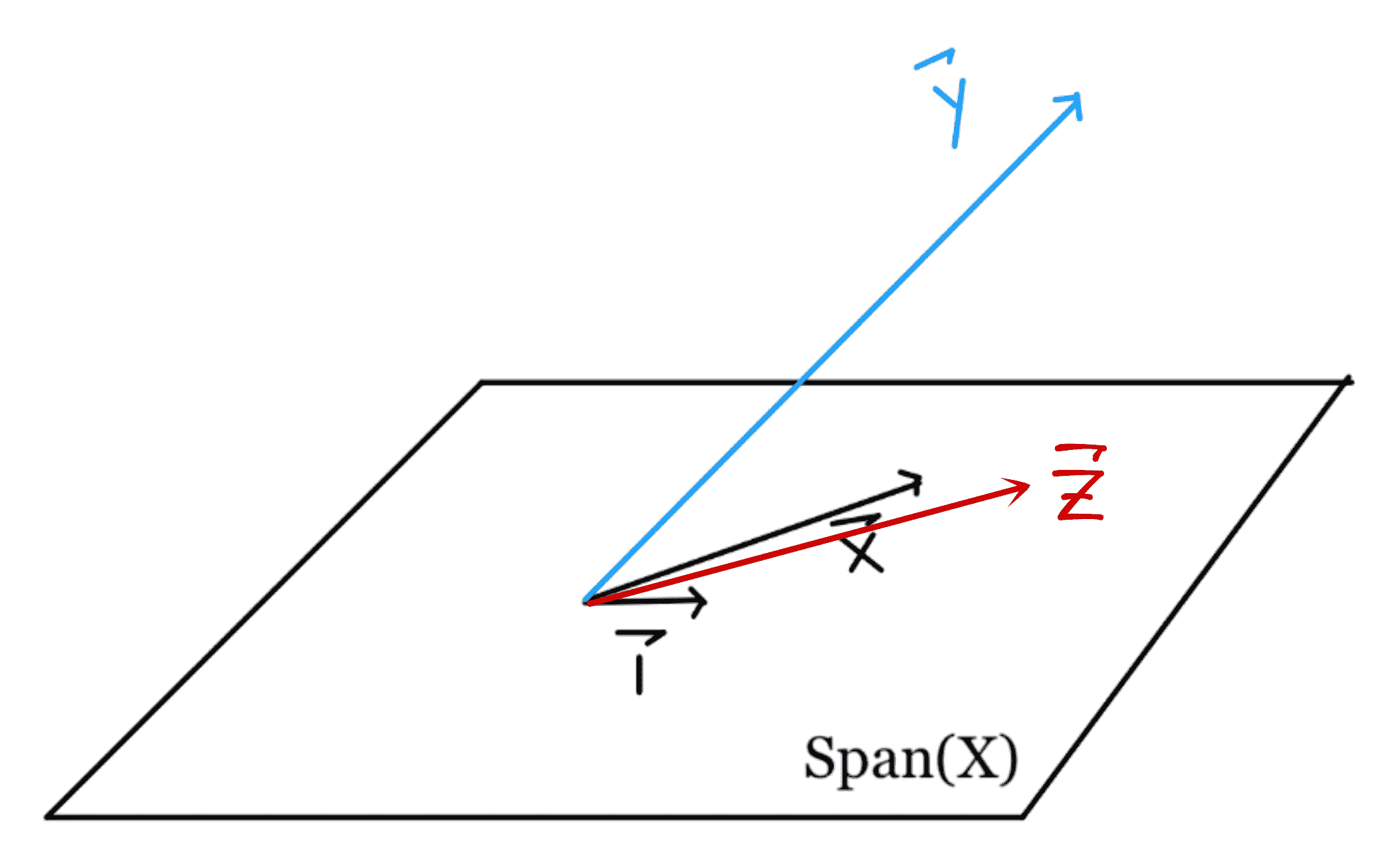因此，我們從查找$\textbf y 的投影轉移到一行：  要查找$\textbf y 到平面上的投影：  現在，讓我們引入另一個變量，$\textbf z$，并顯式地寫出 bias 列： | **Z** | **1** | **X** | **Y** | | --- | --- | --- | --- | | 四 | 1 | 3 | 2 | | 1 | 1 | 0 | 1 | | 0 | 1 | -1 | -2 | 請注意，$\textbf z=\textbf 1+\textbf x$。由于$\textbf z 是$\textbf 1 和$\textbf x 的線性組合，因此它位于原始的$span（\textbf x）中。從形式上講，$\textbf z$與$\ \textbf 1$，$\textbf x$線性相關，并且不會更改$SPAN（\textbf x）$。因此，將$\textbf y$投影到由$\textbf 1$、$\textbf x$、和$\textbf z$所跨越的子空間上，與將$\textbf y$投影到由$\textbf 1 和$\textbf x 所跨越的子空間上相同。  我們也可以通過最小化損失函數來觀察這一點： $$ \begin{aligned} L(\boldsymbol\theta, \textbf{d}, \textbf{y}) &= \left \Vert \qquad \begin{bmatrix} y_1 \\ y_2 \\ y_3 \end{bmatrix} \quad - \quad \begin{bmatrix} 1 & x_1 & z_1 \\ 1 & x_2 & z_2\\ 1 & x_3 & z_3\end{bmatrix} \begin{bmatrix} \theta_0 \\ \theta_1 \\ \theta_2 \end{bmatrix} \qquad \right \Vert ^2 \end{aligned} $$ 我們可能的解決方案如下表：$\Theta_0\textbf 1+\Theta_1\textbf x+Theta_2\textbf z$。 由于$\textbf z=\textbf 1+textbf x$，無論\theta 0$、$\theta 1$和\theta 2$如何，可能的值都可以重寫為： $$ \begin{aligned} \theta_0 \textbf{1} + \theta_1 \textbf{x} + \theta_2 (\textbf{1} + \textbf{x}) &= (\theta_0 + \theta_2) \textbf{1} + (\theta_1 + \theta_2) \textbf{x} \\ \end{aligned} $$ 因此添加$\textbf z$根本不會改變問題。唯一的區別是，我們可以用多種方式表達這個投影。回想一下，我們發現$\textbf y 在由$\textbf 1 和$\textbf x 所橫跨的平面上的投影為： $$ \begin{bmatrix} \textbf{1} & \textbf{x} \end{bmatrix} \begin{bmatrix} - \frac{3}{13} \\ \frac{11}{13} \end{bmatrix} = - \frac{3}{13} \textbf{1} + \frac{11}{13} \textbf{x}$$ 然而，隨著$\textbf z 的引入，我們有更多的方法來表達這個相同的投影向量。 由于$\textbf 1=\textbf z-\textbf x，$\hat \textbf y$也可以表示為： $$ - \frac{3}{13} (\textbf{z} - \textbf{x}) + \frac{11}{13} \textbf{x} = - \frac{3}{13} \textbf{z} + \frac{14}{13} \textbf{x} $$ 由于$\textbf x=\textbf z+textbf 1，$\hat \textbf y$也可以表示為： $$ - \frac{3}{13} \textbf{1} + \frac{11}{13} (\textbf{z} + \textbf{1}) = \frac{8}{13} \textbf{1} + \frac{11}{13} \textbf{z} $$ 但這三個表達式都表示相同的投影。 總之，將線性相關列添加到$\textbf x$不會更改$SPAN（\textbf x）$，因此不會更改投影和最小二乘問題的解決方案。 ## 兩個學派 我們在這節課中把散點圖包括了兩次。第一條提醒我們，像以前一樣，我們正在為數據尋找最合適的行。第二個結果顯示，沒有一條線可以適合所有的點。除了這兩種情況外，我們還試圖用散點圖來破壞我們的矢量空間圖。這是因為散點圖符合最小二乘問題的行空間透視圖：查看每個數據點，并嘗試最小化預測與每個數據之間的距離。在本課中，我們研究了列空間透視圖：每個特征都是一個向量，構建了一個可能的解空間（投影）。 這兩種觀點都是有效的，并且有助于理解，我們希望你看到最小二乘問題的兩面都很有趣！