# 學習 TensorFlow 線性回歸方法 雖然使用矩陣和分解方法非常強大，但 TensorFlow 還有另一種解決斜率和截距的方法。 TensorFlow 可以迭代地執行此操作，逐步學習最小化損失的線性回歸參數。 ## 做好準備 在這個秘籍中，我們將遍歷批量數據點并讓 TensorFlow 更新斜率和`y`截距。我們將使用內置于 scikit-learn 庫中的 iris 數據集，而不是生成的數據。具體來說，我們將通過數據點找到最佳線，其中`x`值是花瓣寬度，`y`值是萼片長度。我們選擇了這兩個，因為它們之間似乎存在線性關系，我們將在最后的繪圖中看到。我們還將在下一節中詳細討論不同損失函數的影響，但對于這個秘籍，我們將使用 L2 損失函數。 ## 操作步驟 我們按如下方式處理秘籍： 1. 我們首先加載必要的庫，創建圖并加載數據： ```py import matplotlib.pyplot as plt import numpy as np import tensorflow as tf from sklearn import datasets from tensorflow.python.framework import ops ops.reset_default_graph() sess = tf.Session() iris = datasets.load_iris() x_vals = np.array([x[3] for x in iris.data]) y_vals = np.array([y[0] for y in iris.data]) ``` 1. 然后我們聲明我們的學習率，批量大小，占位符和模型變量： ```py learning_rate = 0.05 batch_size = 25 x_data = tf.placeholder(shape=[None, 1], dtype=tf.float32) y_target = tf.placeholder(shape=[None, 1], dtype=tf.float32) A = tf.Variable(tf.random_normal(shape=[1,1])) b = tf.Variable(tf.random_normal(shape=[1,1])) ``` 1. 接下來，我們編寫線性模型的公式`y = Ax + b`： ```py model_output = tf.add(tf.matmul(x_data, A), b) ``` 1. 然后，我們聲明我們的 L2 損失函數（包括批量的平均值），初始化變量，并聲明我們的優化器。請注意，我們選擇`0.05`作為我們的學習率： ```py loss = tf.reduce_mean(tf.square(y_target - model_output)) init = tf.global_variables_initializer() sess.run(init) my_opt = tf.train.GradientDescentOptimizer(learning_rate) train_step = my_opt.minimize(loss) ``` 1. 我們現在可以在隨機選擇的批次上循環并訓練模型。我們將運行 100 個循環并每 25 次迭代打印出變量和損失值。請注意，在這里，我們還保存了每次迭代的損失，以便我們以后可以查看它們： ```py loss_vec = [] for i in range(100): rand_index = np.random.choice(len(x_vals), size=batch_size) rand_x = np.transpose([x_vals[rand_index]]) rand_y = np.transpose([y_vals[rand_index]]) sess.run(train_step, feed_dict={x_data: rand_x, y_target: rand_y}) temp_loss = sess.run(loss, feed_dict={x_data: rand_x, y_target: rand_y}) loss_vec.append(temp_loss) if (i+1)%25==0: print('Step #' + str(i+1) + ' A = ' + str(sess.run(A)) + ' b = ' + str(sess.run(b))) print('Loss = ' + str(temp_loss)) Step #25 A = [[ 2.17270374]] b = [[ 2.85338426]] Loss = 1.08116 Step #50 A = [[ 1.70683455]] b = [[ 3.59916329]] Loss = 0.796941 Step #75 A = [[ 1.32762754]] b = [[ 4.08189011]] Loss = 0.466912 Step #100 A = [[ 1.15968263]] b = [[ 4.38497639]] Loss = 0.281003 ``` 1. 接下來，我們將提取我們找到的系數并創建一個最合適的線以放入圖中： ```py [slope] = sess.run(A) [y_intercept] = sess.run(b) best_fit = [] for i in x_vals: best_fit.append(slope*i+y_intercept) ``` 1. 在這里，我們將創建兩個圖。第一個是覆蓋擬合線的數據。第二個是 100 次迭代中的 L2 損失函數。這是生成兩個圖的代碼。 ```py plt.plot(x_vals, y_vals, 'o', label='Data Points') plt.plot(x_vals, best_fit, 'r-', label='Best fit line', linewidth=3) plt.legend(loc='upper left') plt.title('Sepal Length vs Petal Width') plt.xlabel('Petal Width') plt.ylabel('Sepal Length') plt.show() plt.plot(loss_vec, 'k-') plt.title('L2 Loss per Generation') plt.xlabel('Generation') plt.ylabel('L2 Loss') plt.show() ``` 此代碼生成以下擬合數據和損失圖。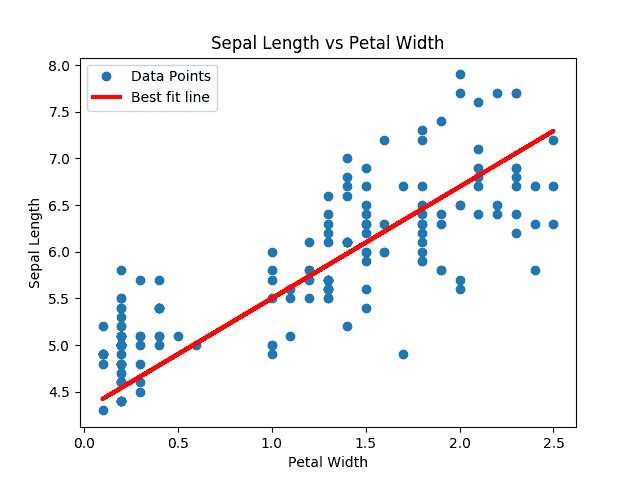  圖 3：來自虹膜數據集的數據點（萼片長度與花瓣寬度）重疊在 TensorFlow 中找到的最佳線條擬合。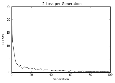  圖 4：用我們的算法擬合數據的 L2 損失;注意損失函數中的抖動，可以通過較大的批量大小減小抖動，或者通過較小的批量大小來增加。 Here is a good place to note how to see whether the model is overfitting or underfitting the data. If our data is broken into test and training sets, and the accuracy is greater on the training set and lower on the test set, then we are overfitting the data. If the accuracy is still increasing on both test and training sets, then the model is underfitting and we should continue training. ## 工作原理 找到的最佳線不保證是最合適的線。最佳擬合線的收斂取決于迭代次數，批量大小，學習率和損失函數。隨著時間的推移觀察損失函數總是很好的做法，因為它可以幫助您解決問題或超參數變化。