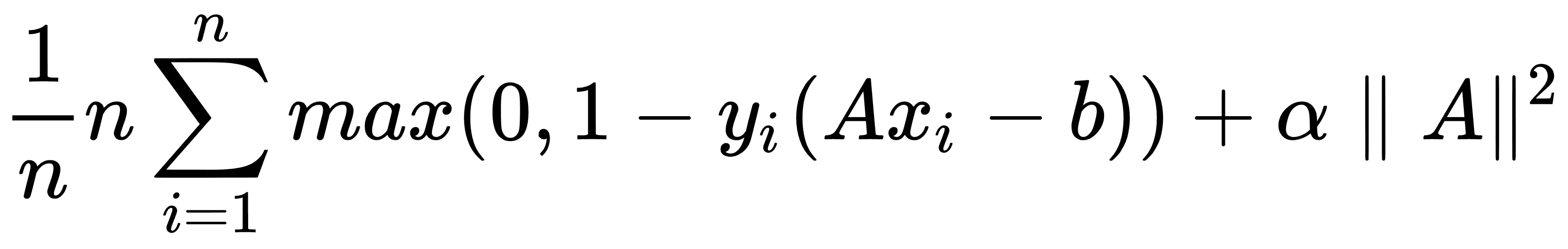
# 使用線性 SVM 對于此示例，我們將從 iris 數據集創建線性分隔符。我們從前面的章節中知道，萼片長度和花瓣寬度創建了一個線性可分的二進制數據集，用于預測花是否是 I. setosa。 ## 做好準備 要在 TensorFlow 中實現軟可分 SVM，我們將實現特定的損失函數，如下所示：  這里，`A`是部分斜率的向量，`b`是截距，`x[i]`是輸入向量，`y[i]`是實際類，（-1 或 1），`α`是軟可分性正則化參數。 ## 操作步驟 我們按如下方式處理秘籍： 1. 我們首先加載必要的庫。這將包括用于訪問虹膜數據集的`scikit-learn`數據集庫。使用以下代碼： ```py import matplotlib.pyplot as plt import numpy as np import tensorflow as tf from sklearn import datasets ``` > 要為此練習設置 scikit-learn，我們只需要輸入`$pip install -U scikit-learn`。請注意，它也安裝了 Anaconda。 1. 接下來，我們啟動圖會話并根據需要加載數據。請記住，我們正在加載虹膜數據集中的第一個和第四個變量，因為它們是萼片長度和萼片寬度。我們正在加載目標變量，對于 I. setosa 將取值 1，否則為-1。使用以下代碼： ```py sess = tf.Session() iris = datasets.load_iris() x_vals = np.array([[x[0], x[3]] for x in iris.data]) y_vals = np.array([1 if y==0 else -1 for y in iris.target]) ``` 1. 我們現在應該將數據集拆分為訓練集和測試集。我們將評估訓練和測試集的準確率。由于我們知道這個數據集是線性可分的，因此我們應該期望在兩個集合上獲得 100％的準確率。要拆分數據，請使用以下代碼： ```py train_indices = np.random.choice(len(x_vals), round(len(x_vals)*0.8), replace=False) test_indices = np.array(list(set(range(len(x_vals))) - set(train_indices))) x_vals_train = x_vals[train_indices] x_vals_test = x_vals[test_indices] y_vals_train = y_vals[train_indices] y_vals_test = y_vals[test_indices] ``` 1. 接下來，我們設置批量大小，占位符和模型變量。值得一提的是，使用這種 SVM 算法，我們需要非常大的批量大小來幫助收斂。我們可以想象，對于非常小的批量大小，最大邊際線會略微跳躍。理想情況下，我們也會慢慢降低學習率，但現在這已經足夠了。此外，`A`變量將采用 2x1 形狀，因為我們有兩個預測變量：萼片長度和花瓣寬度。要進行此設置，我們使用以下代碼： ```py batch_size = 100 x_data = tf.placeholder(shape=[None, 2], dtype=tf.float32) y_target = tf.placeholder(shape=[None, 1], dtype=tf.float32) A = tf.Variable(tf.random_normal(shape=[2,1])) b = tf.Variable(tf.random_normal(shape=[1,1])) ``` 1. 我們現在聲明我們的模型輸出。對于正確分類的點，如果目標是 I. setosa，則返回大于或等于 1 的數字，否則返回小于或等于-1。模型輸出使用以下代碼： ```py model_output = tf.subtract(tf.matmul(x_data, A), b) ``` 1. 接下來，我們將匯總并聲明必要的組件以獲得最大的保證金損失。首先，我們將聲明一個計算向量的 L2 范數的函數。然后，我們添加 margin 參數。然后我們宣布我們的分類損失并將這兩個術語加在一起。使用以下代碼： ```py l2_norm = tf.reduce_sum(tf.square(A)) alpha = tf.constant([0.1]) classification_term = tf.reduce_mean(tf.maximum(0., tf.subtract(1., tf.multiply(model_output, y_target)))) loss = tf.add(classification _term, tf.multiply(alpha, l2_norm)) ``` 1. 現在，我們聲明我們的預測和準確率函數，以便我們可以評估訓練集和測試集的準確率，如下所示： ```py prediction = tf.sign(model_output) accuracy = tf.reduce_mean(tf.cast(tf.equal(prediction, y_target), tf.float32)) ``` 1. 在這里，我們將聲明我們的優化函數并初始化我們的模型變量;我們在以下代碼中執行此操作： ```py my_opt = tf.train.GradientDescentOptimizer(0.01) train_step = my_opt.minimize(loss) init = tf.global_variables_initializer() sess.run(init) ``` 1. 我們現在可以開始我們的訓練循環，記住我們想要在訓練和測試集上記錄我們的損失和訓練準確率，如下所示： ```py loss_vec = [] train_accuracy = [] test_accuracy = [] for i in range(500): rand_index = np.random.choice(len(x_vals_train), size=batch_size) rand_x = x_vals_train[rand_index] rand_y = np.transpose([y_vals_train[rand_index]]) sess.run(train_step, feed_dict={x_data: rand_x, y_target: rand_y}) temp_loss = sess.run(loss, feed_dict={x_data: rand_x, y_target: rand_y}) loss_vec.append(temp_loss) train_acc_temp = sess.run(accuracy, feed_dict={x_data: x_vals_train, y_target: np.transpose([y_vals_train])}) train_accuracy.append(train_acc_temp) test_acc_temp = sess.run(accuracy, feed_dict={x_data: x_vals_test, y_target: np.transpose([y_vals_test])}) test_accuracy.append(test_acc_temp) if (i+1)%100==0: print('Step #' + str(i+1) + ' A = ' + str(sess.run(A)) + ' b = ' + str(sess.run(b))) print('Loss = ' + str(temp_loss)) ``` 1. 訓練期間腳本的輸出應如下所示： ```py Step #100 A = [[-0.10763293] [-0.65735245]] b = [[-0.68752676]] Loss = [ 0.48756418] Step #200 A = [[-0.0650763 ] [-0.89443302]] b = [[-0.73912662]] Loss = [ 0.38910741] Step #300 A = [[-0.02090022] [-1.12334013]] b = [[-0.79332656]] Loss = [ 0.28621092] Step #400 A = [[ 0.03189624] [-1.34912157]] b = [[-0.8507266]] Loss = [ 0.22397576] Step #500 A = [[ 0.05958777] [-1.55989814]] b = [[-0.9000265]] Loss = [ 0.20492229] ``` 1. 為了繪制輸出（擬合，損失和精度），我們必須提取系數并將`x`值分成 I. setosa 和 Non-setosa，如下所示： ```py [[a1], [a2]] = sess.run(A) [[b]] = sess.run(b) slope = -a2/a1 y_intercept = b/a1 x1_vals = [d[1] for d in x_vals] best_fit = [] for i in x1_vals: best_fit.append(slope*i+y_intercept) setosa_x = [d[1] for i,d in enumerate(x_vals) if y_vals[i]==1] setosa_y = [d[0] for i,d in enumerate(x_vals) if y_vals[i]==1] not_setosa_x = [d[1] for i,d in enumerate(x_vals) if y_vals[i]==-1] not_setosa_y = [d[0] for i,d in enumerate(x_vals) if y_vals[i]==-1] ``` 1. 以下是使用線性分離器擬合，精度和損耗繪制數據的代碼： ```py plt.plot(setosa_x, setosa_y, 'o', label='I. setosa') plt.plot(not_setosa_x, not_setosa_y, 'x', label='Non-setosa') plt.plot(x1_vals, best_fit, 'r-', label='Linear Separator', linewidth=3) plt.ylim([0, 10]) plt.legend(loc='lower right') plt.title('Sepal Length vs Petal Width') plt.xlabel('Petal Width') plt.ylabel('Sepal Length') plt.show() plt.plot(train_accuracy, 'k-', label='Training Accuracy') plt.plot(test_accuracy, 'r--', label='Test Accuracy') plt.title('Train and Test Set Accuracies') plt.xlabel('Generation') plt.ylabel('Accuracy') plt.legend(loc='lower right') plt.show() plt.plot(loss_vec, 'k-') plt.title('Loss per Generation') plt.xlabel('Generation') plt.ylabel('Loss') plt.show() ``` > 以這種方式使用 TensorFlow 來實現 SVD 算法可能導致每次運行的結果略有不同。其原因包括隨機訓練/測試集拆分以及每個訓練批次中不同批次點的選擇。此外，在每一代之后慢慢降低學習率是理想的。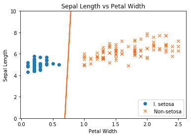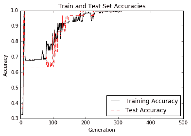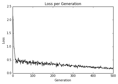 得到的圖如下：  圖 2：最終線性 SVM 與繪制的兩個類別擬合  圖 3：迭代測試和訓練集精度;我們確實獲得 100％的準確率，因為這兩個類是線性可分的  圖 4：超過 500 次迭代的最大邊際損失圖 ## 工作原理 在本文中，我們已經證明使用最大邊際損失函數可以實現線性 SVD 模型。