# 使用最近鄰進行圖像識別 最近鄰也可用于圖像識別。圖像識別數據集的問題世界是 MNIST 手寫數字數據集。由于我們將在后面的章節中將此數據集用于各種神經網絡圖像識別算法，因此將結果與非神經網絡算法進行比較將會很棒。 ## 做好準備 MNIST 數字數據集由數千個尺寸為 28×28 像素的標記圖像組成。雖然這被認為是一個小圖像，但它對于最近鄰算法總共有 784 個像素（或特征）。我們將通過考慮最近的`k`鄰居（`k=4`，在該示例中）的模式預測來計算該分類問題的最近鄰預測。 ## 操作步驟 我們將按如下方式處理秘籍： 1. 我們將從加載必要的庫開始。請注意，我們還將導入 Python 圖像庫（PIL），以便能夠繪制預測輸出的樣本。 TensorFlow 有一個內置方法來加載我們將使用的 MNIST 數據集，如下所示： ```py import random import numpy as np import tensorflow as tf import matplotlib.pyplot as plt from PIL import Image from tensorflow.examples.tutorials.mnist import input_data ``` 1. 現在，我們將啟動圖會話并以單熱編碼形式加載 MNIST 數據： ```py sess = tf.Session() mnist = input_data.read_data_sets("MNIST_data/", one_hot=True) ``` > 單熱編碼是更適合數值計算的分類值的數值表示。這里，我們有 10 個類別（數字 0-9），并將它們表示為長度為 10 的 0-1 向量。例如，0 類別由向量 1,0,0,0,0,0 表示， 0,0,0,0,1 向量用 0,1,0,0,0,0,0,0,0,0 表示，依此類推。 1. 因為 MNIST 數據集很大并且計算數萬個輸入上的 784 個特征之間的距離在計算上是困難的，所以我們將采樣一組較小的圖像來訓練。此外，我們將選擇一個可被 6 整除的測試集編號，僅用于繪圖目的，因為我們將繪制最后一批六個圖像以查看結果的示例： ```py train_size = 1000 test_size = 102 rand_train_indices = np.random.choice(len(mnist.train.images), train_size, replace=False) rand_test_indices = np.random.choice(len(mnist.test.images), test_size, replace=False) x_vals_train = mnist.train.images[rand_train_indices] x_vals_test = mnist.test.images[rand_test_indices] y_vals_train = mnist.train.labels[rand_train_indices] y_vals_test = mnist.test.labels[rand_test_indices] ``` 1. 我們將聲明我們的`k`值和批量大小： ```py k = 4 batch_size=6 ``` 1. 現在，我們將初始化將添加到圖中的占位符： ```py x_data_train = tf.placeholder(shape=[None, 784], dtype=tf.float32) x_data_test = tf.placeholder(shape=[None, 784], dtype=tf.float32) y_target_train = tf.placeholder(shape=[None, 10], dtype=tf.float32) y_target_test = tf.placeholder(shape=[None, 10], dtype=tf.float32) ``` 1. 然后我們將聲明我們的距離度量。在這里，我們將使用 L1 度量（絕對值）： ```py distance = tf.reduce_sum(tf.abs(tf.subtract(x_data_train, tf.expand_dims(x_data_test,1))), reduction_indices=2) ``` > 請注意，我們也可以使用以下代碼來改變距離函數：`distance = tf.sqrt(tf.reduce_sum(tf.square(tf.subtract(x_data_train, tf.expand_dims(x_data_test,1))), reduction_indices=1))`。 1. 現在，我們將找到最接近的頂級`k`圖像并預測模式。該模式將在單熱編碼索引上執行，計數最多： ```py top_k_xvals, top_k_indices = tf.nn.top_k(tf.negative(distance), k=k) prediction_indices = tf.gather(y_target_train, top_k_indices) count_of_predictions = tf.reduce_sum(prediction_indices, reduction_indices=1) prediction = tf.argmax(count_of_predictions) ``` 1. 我們現在可以遍歷我們的測試集，計算預測并存儲它們，如下所示： ```py num_loops = int(np.ceil(len(x_vals_test)/batch_size)) test_output = [] actual_vals = [] for i in range(num_loops): min_index = i*batch_size max_index = min((i+1)*batch_size,len(x_vals_train)) x_batch = x_vals_test[min_index:max_index] y_batch = y_vals_test[min_index:max_index] predictions = sess.run(prediction, feed_dict={x_data_train: x_vals_train, x_data_test: x_batch, y_target_train: y_vals_train, y_target_test: y_batch}) test_output.extend(predictions) actual_vals.extend(np.argmax(y_batch, axis=1)) ``` 1. 現在我們已經保存了實際和預測的輸出，我們可以計算出準確率。由于我們對測試/訓練數據集進行隨機抽樣，這會發生變化，但最終我們的準確率值應該在 80％-90％左右： ```py accuracy = sum([1./test_size for i in range(test_size) if test_output[i]==actual_vals[i]]) print('Accuracy on test set: ' + str(accuracy)) Accuracy on test set: 0.8333333333333325 ``` 1. 以下是繪制前面批量結果的代碼： ```py actuals = np.argmax(y_batch, axis=1) Nrows = 2 Ncols = 3 for i in range(len(actuals)): plt.subplot(Nrows, Ncols, i+1) plt.imshow(np.reshape(x_batch[i], [28,28]), cmap='Greys_r') plt.title('Actual: ' + str(actuals[i]) + ' Pred: ' + str(predictions[i]), fontsize=10) frame = plt.gca() frame.axes.get_xaxis().set_visible(False) frame.axes.get_yaxis().set_visible(False) ``` 結果如下：  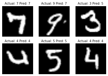圖 4：我們運行最近鄰預測的最后一批六個圖像。我們可以看到，我們并沒有完全正確地獲得所有圖像。 ## 工作原理 給定足夠的計算時間和計算資源，我們可以使測試和訓練集更大。這可能會提高我們的準確率，也是防止過擬合的常用方法。另外，請注意，此算法需要進一步探索理想的`k`值進行選擇。可以在數據集上進行一組交叉驗證實驗后選擇`k`值。 ## 更多 我們還可以使用最近鄰居算法來評估用戶看不見的數字。有關使用此模型評估用戶輸入數字的方法，請參閱在線倉庫，地址為 [https://github.com/nfmcclure/tensorflow_cookbook](https://github.com/nfmcclure/tensorflow_cookbook) 。 在本章中，我們探討了如何使用 k-NN 算法進行回歸和分類。我們討論了距離函數的不同用法，以及如何將它們混合在一起。我們鼓勵讀者探索不同的距離度量，權重和`k`值，以優化這些方法的準確率。