# 訓練 Siamese RNN 相似性度量 與許多其他模型相比，RNN 模型的一個重要特性是它們可以處理各種長度的序列。利用這一點，以及它們可以推廣到之前未見過的序列這一事實，我們可以創建一種方法來衡量輸入的相似序列是如何相互作用的。在這個秘籍中，我們將訓練一個 Siamese 相似性 RNN 來測量地址之間的相似性以進行記錄匹配。 ## 做好準備 在本文中，我們將構建一個雙向 RNN 模型，該模型將輸入到一個完全連接的層，該層輸出一個固定長度的數值向量。我們為兩個輸入地址創建雙向 RNN 層，并將輸出饋送到完全連接的層，該層輸出固定長度的數字向量（長度 100）。然后我們將兩個向量輸出與余弦距離進行比較，余弦距離在-1 和 1 之間。我們將輸入數據表示為與目標 1 相似，并且目標為-1。余弦距離的預測只是輸出的符號（負值表示不相似，正表示相似）。我們可以使用此網絡通過從查詢地址獲取在余弦距離上得分最高的參考地址來進行記錄匹配。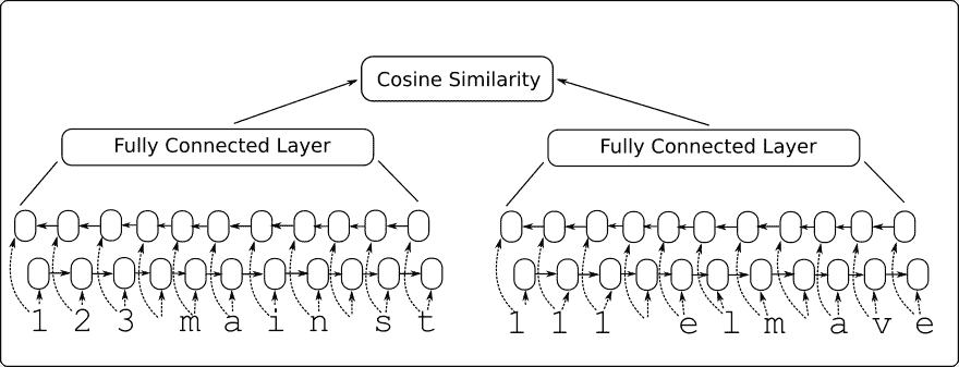 請參閱以下網絡架構圖：  圖 8：Siamese RNN 相似性模型架構 這個模型的優點還在于它接受以前沒有見過的輸入，并且可以將它們與-1 到 1 的輸出進行比較。我們將通過選擇模型之前未見過的測試地址在代碼中顯示它并查看它是否可以匹配到類似的地址。 ## 操作步驟 1. 我們首先加載必要的庫并開始圖會話： ```py import os import random import string import numpy as np import matplotlib.pyplot as plt import tensorflow as tf sess = tf.Session() ``` 1. 我們現在設置模型參數如下： ```py batch_size = 200 n_batches = 300 max_address_len = 20 margin = 0.25 num_features = 50 dropout_keep_prob = 0.8 ``` 1. 接下來，我們創建 Siamese RNN 相似性模型類，如下所示： ```py def snn(address1, address2, dropout_keep_prob, vocab_size, num_features, input_length): # Define the Siamese double RNN with a fully connected layer at the end def Siamese_nn(input_vector, num_hidden): cell_unit = tf.nn.rnn_cell.BasicLSTMCell # Forward direction cell lstm_forward_cell = cell_unit(num_hidden, forget_bias=1.0) lstm_forward_cell = tf.nn.rnn_cell.DropoutWrapper(lstm_forward_cell, output_keep_prob=dropout_keep_prob) # Backward direction cell lstm_backward_cell = cell_unit(num_hidden, forget_bias=1.0) lstm_backward_cell = tf.nn.rnn_cell.DropoutWrapper(lstm_backward_cell, output_keep_prob=dropout_keep_prob) # Split title into a character sequence input_embed_split = tf.split(1, input_length, input_vector) input_embed_split = [tf.squeeze(x, squeeze_dims=[1]) for x in input_embed_split] # Create bidirectional layer outputs, _, _ = tf.nn.bidirectional_rnn(lstm_forward_cell, lstm_backward_cell, input_embed_split, dtype=tf.float32) # Average The output over the sequence temporal_mean = tf.add_n(outputs) / input_length # Fully connected layer output_size = 10 A = tf.get_variable(name="A", shape=[2*num_hidden, output_size], dtype=tf.float32, initializer=tf.random_normal_initializer(stddev=0.1)) b = tf.get_variable(name="b", shape=[output_size], dtype=tf.float32, initializer=tf.random_normal_initializer(stddev=0.1)) final_output = tf.matmul(temporal_mean, A) + b final_output = tf.nn.dropout(final_output, dropout_keep_prob) return(final_output) with tf.variable_scope("Siamese") as scope: output1 = Siamese_nn(address1, num_features) # Declare that we will use the same variables on the second string scope.reuse_variables() output2 = Siamese_nn(address2, num_features) # Unit normalize the outputs output1 = tf.nn.l2_normalize(output1, 1) output2 = tf.nn.l2_normalize(output2, 1) # Return cosine distance # in this case, the dot product of the norms is the same. dot_prod = tf.reduce_sum(tf.mul(output1, output2), 1) return dot_prod ``` > 請注意，使用變量范圍在兩個地址輸入的 Siamese 網絡的兩個部分之間共享參數。另外，請注意，余弦距離是通過歸一化向量的點積來實現的。 1. 現在我們將聲明我們的預測函數，它只是余弦距離的符號，如下所示： ```py def get_predictions(scores): predictions = tf.sign(scores, name="predictions") return predictions ``` 1. 現在我們將如前所述聲明我們的`loss`函數。請記住，我們希望為錯誤留下邊距（類似于 SVM 模型）。我們還將有一個真正的積極和真正的消極的損失期限。使用以下代碼進行損失： ```py def loss(scores, y_target, margin): # Calculate the positive losses pos_loss_term = 0.25 * tf.square(tf.sub(1., scores)) pos_mult = tf.cast(y_target, tf.float32) # Make sure positive losses are on similar strings positive_loss = tf.mul(pos_mult, pos_loss_term) # Calculate negative losses, then make sure on dissimilar strings neg_mult = tf.sub(1., tf.cast(y_target, tf.float32)) negative_loss = neg_mult*tf.square(scores) # Combine similar and dissimilar losses loss = tf.add(positive_loss, negative_loss) # Create the margin term. This is when the targets are 0, and the scores are less than m, return 0\. # Check if target is zero (dissimilar strings) target_zero = tf.equal(tf.cast(y_target, tf.float32), 0.) # Check if cosine outputs is smaller than margin less_than_margin = tf.less(scores, margin) # Check if both are true both_logical = tf.logical_and(target_zero, less_than_margin) both_logical = tf.cast(both_logical, tf.float32) # If both are true, then multiply by (1-1)=0\. multiplicative_factor = tf.cast(1\. - both_logical, tf.float32) total_loss = tf.mul(loss, multiplicative_factor) # Average loss over batch avg_loss = tf.reduce_mean(total_loss) return avg_loss ``` 1. 我們聲明`accuracy`函數如下： ```py def accuracy(scores, y_target): predictions = get_predictions(scores) correct_predictions = tf.equal(predictions, y_target) accuracy = tf.reduce_mean(tf.cast(correct_predictions, tf.float32)) return accuracy ``` 1. 我們將通過在地址中創建拼寫錯誤來創建類似的地址。我們將這些地址（參考地址和拼寫錯誤地址）表示為類似： ```py def create_typo(s): rand_ind = random.choice(range(len(s))) s_list = list(s) s_list[rand_ind]=random.choice(string.ascii_lowercase + '0123456789') s = ''.join(s_list) return s ``` 1. 我們將生成的數據將是街道號碼，`street_names`和街道后綴的隨機組合。名稱和后綴來自以下列表： ```py street_names = ['abbey', 'baker', 'canal', 'donner', 'elm', 'fifth', 'grandvia', 'hollywood', 'interstate', 'jay', 'kings'] street_types = ['rd', 'st', 'ln', 'pass', 'ave', 'hwy', 'cir', 'dr', 'jct'] ``` 1. 我們生成測試查詢和引用如下： ```py test_queries = ['111 abbey ln', '271 doner cicle', '314 king avenue', 'tensorflow is fun'] test_references = ['123 abbey ln', '217 donner cir', '314 kings ave', '404 hollywood st', 'tensorflow is so fun'] ``` > 請注意，最后一個查詢和引用不是模型之前會看到的地址，但我們希望它們將是模型最終看到的最相似的地址。 1. 我們現在將定義如何生成一批數據。我們的批量數據將是 50％類似的地址（參考地址和拼寫錯誤地址）和 50％不同的地址。我們通過占用地址列表的一半并將目標移動一個位置（使用`numpy.roll()`函數）來生成不同的地址： ```py def get_batch(n): # Generate a list of reference addresses with similar addresses that have # a typo. numbers = [random.randint(1, 9999) for i in range(n)] streets = [random.choice(street_names) for i in range(n)] street_suffs = [random.choice(street_types) for i in range(n)] full_streets = [str(w) + ' ' + x + ' ' + y for w,x,y in zip(numbers, streets, street_suffs)] typo_streets = [create_typo(x) for x in full_streets] reference = [list(x) for x in zip(full_streets, typo_streets)] # Shuffle last half of them for training on dissimilar addresses half_ix = int(n/2) bottom_half = reference[half_ix:] true_address = [x[0] for x in bottom_half] typo_address = [x[1] for x in bottom_half] typo_address = list(np.roll(typo_address, 1)) bottom_half = [[x,y] for x,y in zip(true_address, typo_address)] reference[half_ix:] = bottom_half # Get target similarities (1's for similar, -1's for non-similar) target = [1]*(n-half_ix) + [-1]*half_ix reference = [[x,y] for x,y in zip(reference, target)] return reference ``` 1. 接下來，我們定義地址詞匯表并指定如何將地址熱編碼為索引： ```py vocab_chars = string.ascii_lowercase + '0123456789 ' vocab2ix_dict = {char:(ix+1) for ix, char in enumerate(vocab_chars)} vocab_length = len(vocab_chars) + 1 # Define vocab one-hot encoding def address2onehot(address, vocab2ix_dict = vocab2ix_dict, max_address_len = max_address_len): # translate address string into indices address_ix = [vocab2ix_dict[x] for x in list(address)] # Pad or crop to max_address_len address_ix = (address_ix + [0]*max_address_len)[0:max_address_len] return address_ix ``` 1. 處理完詞匯后，我們將開始聲明我們的模型占位符和嵌入查找。對于嵌入查找，我們將使用單一矩陣作為查找矩陣來使用單熱編碼嵌入。使用以下代碼： ```py address1_ph = tf.placeholder(tf.int32, [None, max_address_len], name="address1_ph") address2_ph = tf.placeholder(tf.int32, [None, max_address_len], name="address2_ph") y_target_ph = tf.placeholder(tf.int32, [None], name="y_target_ph") dropout_keep_prob_ph = tf.placeholder(tf.float32, name="dropout_keep_prob") # Create embedding lookup identity_mat = tf.diag(tf.ones(shape=[vocab_length])) address1_embed = tf.nn.embedding_lookup(identity_mat, address1_ph) address2_embed = tf.nn.embedding_lookup(identity_mat, address2_ph) ``` 1. 我們現在將聲明`model`，`batch_accuracy`，`batch_loss`和`predictions`操作如下： ```py # Define Model text_snn = model.snn(address1_embed, address2_embed, dropout_keep_prob_ph, vocab_length, num_features, max_address_len) # Define Accuracy batch_accuracy = model.accuracy(text_snn, y_target_ph) # Define Loss batch_loss = model.loss(text_snn, y_target_ph, margin) # Define Predictions predictions = model.get_predictions(text_snn) ``` 1. 最后，在我們開始訓練之前，我們將優化和初始化操作添加到圖中，如下所示： ```py # Declare optimizer optimizer = tf.train.AdamOptimizer(0.01) # Apply gradients train_op = optimizer.minimize(batch_loss) # Initialize Variables init = tf.global_variables_initializer() sess.run(init) ``` 1. 我們現在將遍歷訓練世代并跟蹤損失和準確率： ```py train_loss_vec = [] train_acc_vec = [] for b in range(n_batches): # Get a batch of data batch_data = get_batch(batch_size) # Shuffle data np.random.shuffle(batch_data) # Parse addresses and targets input_addresses = [x[0] for x in batch_data] target_similarity = np.array([x[1] for x in batch_data]) address1 = np.array([address2onehot(x[0]) for x in input_addresses]) address2 = np.array([address2onehot(x[1]) for x in input_addresses]) train_feed_dict = {address1_ph: address1, address2_ph: address2, y_target_ph: target_similarity, dropout_keep_prob_ph: dropout_keep_prob} _, train_loss, train_acc = sess.run([train_op, batch_loss, batch_accuracy], feed_dict=train_feed_dict) # Save train loss and accuracy train_loss_vec.append(train_loss) train_acc_vec.append(train_acc) ``` 1. 經過訓練，我們現在處理測試查詢和引用，以了解模型的執行方式： ```py test_queries_ix = np.array([address2onehot(x) for x in test_queries]) test_references_ix = np.array([address2onehot(x) for x in test_references]) num_refs = test_references_ix.shape[0] best_fit_refs = [] for query in test_queries_ix: test_query = np.repeat(np.array([query]), num_refs, axis=0) test_feed_dict = {address1_ph: test_query, address2_ph: test_references_ix, y_target_ph: target_similarity, dropout_keep_prob_ph: 1.0} test_out = sess.run(text_snn, feed_dict=test_feed_dict) best_fit = test_references[np.argmax(test_out)] best_fit_refs.append(best_fit) print('Query Addresses: {}'.format(test_queries)) print('Model Found Matches: {}'.format(best_fit_refs)) ``` 1. 這導致以下輸出： ```py Query Addresses: ['111 abbey ln', '271 doner cicle', '314 king avenue', 'tensorflow is fun'] Model Found Matches: ['123 abbey ln', '217 donner cir', '314 kings ave', 'tensorflow is so fun'] ``` ## 更多 我們可以從測試查詢和參考中看到模型不僅能夠識別正確的參考地址，而且還能夠推廣到非地址短語。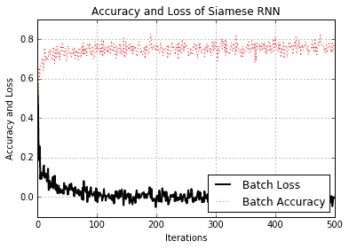我們還可以通過查看訓練期間的損失和準確率來了解模型的執行情況：  圖 9：訓練期間 Siamese RNN 相似性模型的準確率和損失 請注意，我們沒有為此練習指定測試集。這是因為我們如何生成數據。我們創建了一個批量函數，每次調用它時都會創建新的批量數據，因此模型始終可以看到新數據。因此，我們可以使用批量損失和精度作為測試損失和準確率的替代項。但是，對于一組有限的實際數據，情況永遠不會如此，因為我們總是需要訓練和測試集來判斷模型的表現。