# 改進線性模型的預測 在前面的秘籍中，我們注意到我們擬合的參數數量遠遠超過等效的線性模型。在這個秘籍中，我們將嘗試通過使用神經網絡來改進我們的低出生體重的邏輯模型。 ## 做好準備 對于這個秘籍，我們將加載低出生體重數據，并使用神經網絡與兩個隱藏的完全連接的層與乙狀結腸激活，以適應低出生體重的概率。 ## 怎么做 我們按如下方式處理秘籍： 1. 我們首先加載庫并初始化我們的計算圖，如下所示： ```py import matplotlib.pyplot as plt import numpy as np import tensorflow as tf import requests sess = tf.Session() ``` 1. 接下來，我們按照前面的秘籍加載，提取和標準化我們的數據，除了在這里我們將使用低出生體重指示變量作為我們的目標而不是實際出生體重，如下所示： ```py # Name of data file birth_weight_file = 'birth_weight.csv' birthdata_url = 'https://github.com/nfmcclure/tensorflow_cookbook/raw/master' \ '/01_Introduction/07_Working_with_Data_Sources/birthweight_data/birthweight.dat' # Download data and create data file if file does not exist in current directory if not os.path.exists(birth_weight_file): birth_file = requests.get(birthdata_url) birth_data = birth_file.text.split('\r\n') birth_header = birth_data[0].split('\t') birth_data = [[float(x) for x in y.split('\t') if len(x) >= 1] for y in birth_data[1:] if len(y) >= 1] with open(birth_weight_file, "w") as f: writer = csv.writer(f) writer.writerows([birth_header]) writer.writerows(birth_data) # read birth weight data into memory birth_data = [] with open(birth_weight_file, newline='') as csvfile: csv_reader = csv.reader(csvfile) birth_header = next(csv_reader) for row in csv_reader: birth_data.append(row) birth_data = [[float(x) for x in row] for row in birth_data] # Pull out target variable y_vals = np.array([x[0] for x in birth_data]) # Pull out predictor variables (not id, not target, and not birthweight) x_vals = np.array([x[1:8] for x in birth_data]) train_indices = np.random.choice(len(x_vals), round(len(x_vals)*0.8), replace=False) test_indices = np.array(list(set(range(len(x_vals))) - set(train_indices))) x_vals_train = x_vals[train_indices] x_vals_test = x_vals[test_indices] y_vals_train = y_vals[train_indices] y_vals_test = y_vals[test_indices] def normalize_cols(m, col_min=np.array([None]), col_max=np.array([None])): if not col_min[0]: col_min = m.min(axis=0) if not col_max[0]: col_max = m.max(axis=0) return (m - col_min) / (col_max - col_min), col_min, col_max x_vals_train, train_min, train_max = np.nan_to_num(normalize_cols(x_vals_train)) x_vals_test, _, _ = np.nan_to_num(normalize_cols(x_vals_test, train_min, train_max)) ``` 1. 接下來，我們需要聲明我們的批量大小和數據的占位符，如下所示： ```py batch_size = 90 x_data = tf.placeholder(shape=[None, 7], dtype=tf.float32) y_target = tf.placeholder(shape=[None, 1], dtype=tf.float32) ``` 1. 如前所述，我們現在需要聲明在模型中初始化變量和層的函數。為了創建更好的邏輯函數，我們需要創建一個在輸入層上返回邏輯層的函數。換句話說，我們將使用完全連接的層并為每個層返回一個 sigmoid 元素。重要的是要記住我們的損失函數將包含最終的 sigmoid，因此我們要在最后一層指定我們不會返回輸出的 sigmoid，如下所示： ```py def init_variable(shape): return tf.Variable(tf.random_normal(shape=shape)) # Create a logistic layer definition def logistic(input_layer, multiplication_weight, bias_weight, activation = True): linear_layer = tf.add(tf.matmul(input_layer, multiplication_weight), bias_weight) if activation: return tf.nn.sigmoid(linear_layer) else: return linear_layer ``` 1. 現在我們將聲明三個層（兩個隱藏層和一個輸出層）。我們將首先為每個層初始化權重和偏差矩陣，并按如下方式定義層操作： ```py # First logistic layer (7 inputs to 14 hidden nodes) A1 = init_variable(shape=[7,14]) b1 = init_variable(shape=[14]) logistic_layer1 = logistic(x_data, A1, b1) # Second logistic layer (14 hidden inputs to 5 hidden nodes) A2 = init_variable(shape=[14,5]) b2 = init_variable(shape=[5]) logistic_layer2 = logistic(logistic_layer1, A2, b2) # Final output layer (5 hidden nodes to 1 output) A3 = init_variable(shape=[5,1]) b3 = init_variable(shape=[1]) final_output = logistic(logistic_layer2, A3, b3, activation=False) ``` 1. 接下來，我們聲明我們的損失（交叉熵）和優化算法，并初始化以下變量： ```py # Create loss function loss = tf.reduce_mean(tf.nn.sigmoid_cross_entropy_with_logits(logits=final_output, labels=y_target)) # Declare optimizer my_opt = tf.train.AdamOptimizer(learning_rate = 0.002) train_step = my_opt.minimize(loss) # Initialize variables init = tf.global_variables_initializer() sess.run(init) ``` > 交叉熵是一種測量概率之間距離的方法。在這里，我們想要測量確定性（0 或 1）與模型概率（`0<x<1`）之間的差異。 TensorFlow 使用內置的 sigmoid 函數實現交叉熵。這也是超參數調整的一部分，因為我們更有可能找到最佳的損失函數，學習率和針對當前問題的優化算法。為簡潔起見，我們不包括超參數調整。 1. 為了評估和比較我們的模型與以前的模型，我們需要在圖上創建預測和精度操作。這將允許我們提供整個測試集并確定準確率，如下所示： ```py prediction = tf.round(tf.nn.sigmoid(final_output)) predictions_correct = tf.cast(tf.equal(prediction, y_target), tf.float32) accuracy = tf.reduce_mean(predictions_correct) ``` 1. 我們現在準備開始我們的訓練循環。我們將訓練 1500 代并保存模型損失并訓練和測試精度以便以后進行繪圖。我們的訓練循環使用以下代碼啟動： ```py # Initialize loss and accuracy vectors loss_vec = [] train_acc = [] test_acc = [] for i in range(1500): # Select random indicies for batch selection rand_index = np.random.choice(len(x_vals_train), size=batch_size) # Select batch rand_x = x_vals_train[rand_index] rand_y = np.transpose([y_vals_train[rand_index]]) # Run training step sess.run(train_step, feed_dict={x_data: rand_x, y_target: rand_y}) # Get training loss temp_loss = sess.run(loss, feed_dict={x_data: rand_x, y_target: rand_y}) loss_vec.append(temp_loss) # Get training accuracy temp_acc_train = sess.run(accuracy, feed_dict={x_data: x_vals_train, y_target: np.transpose([y_vals_train])}) train_acc.append(temp_acc_train) # Get test accuracy temp_acc_test = sess.run(accuracy, feed_dict={x_data: x_vals_test, y_target: np.transpose([y_vals_test])}) test_acc.append(temp_acc_test) if (i+1)%150==0: print('Loss = '' + str(temp_loss)) ``` 1. 上一步應該產生以下輸出： ```py Loss = 0.696393 Loss = 0.591708 Loss = 0.59214 Loss = 0.505553 Loss = 0.541974 Loss = 0.512707 Loss = 0.590149 Loss = 0.502641 Loss = 0.518047 Loss = 0.502616 ``` 1. 以下代碼塊說明了如何使用`matplotlib`繪制交叉熵損失以及訓練和測試集精度： ```py # Plot loss over time plt.plot(loss_vec, 'k-') plt.title('Cross Entropy Loss per Generation') plt.xlabel('Generation') plt.ylabel('Cross Entropy Loss') plt.show() # Plot train and test accuracy plt.plot(train_acc, 'k-', label='Train Set Accuracy') plt.plot(test_acc, 'r--', label='Test Set Accuracy') plt.title('Train and Test Accuracy') plt.xlabel('Generation') plt.ylabel('Accuracy') plt.legend(loc='lower right') plt.show() ``` 我們得到每代交叉熵損失的圖如下：  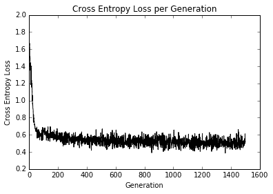圖 7：超過 1500 次迭代的訓練損失 在大約 50 代之內，我們已經達到了良好的模式。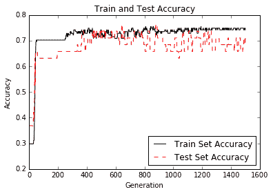在我們繼續訓練時，我們可以看到在剩余的迭代中獲得的很少，如下圖所示：  圖 8：訓練組和測試裝置的準確率 正如您在上圖中所看到的，我們很快就找到了一個好模型。 ## 工作原理 在考慮使用神經網絡建模數據時，您必須考慮優缺點。雖然我們的模型比以前的模型融合得更快，并且可能具有更高的準確率，但這需要付出代價;我們正在訓練更多的模型變量，并且更有可能過擬合。為了檢查是否發生過擬合，我們會查看測試和訓練集的準確率。如果訓練集的準確率繼續增加而測試集的精度保持不變或甚至略微下降，我們可以假設過擬合正在發生。 為了對抗欠擬合，我們可以增加模型深度或訓練模型以進行更多迭代。為了解決過擬合問題，我們可以為模型添加更多數據或添加正則化技術。 同樣重要的是要注意我們的模型變量不像線性模型那樣可解釋。神經網絡模型具有比線性模型更難解釋的系數，因為它們解釋了模型中特征的重要性。