# 實現簡單的 CNN 在本文中，我們將開發一個四層卷積神經網絡，以提高我們預測 MNIST 數字的準確率。前兩個卷積層將各自由卷積-ReLU-Max 池操作組成，最后兩個層將是完全連接的層。 ## 做好準備 為了訪問 MNIST 數據，TensorFlow 有一個`examples.tutorials`包，它具有很好的數據集加載函數。加載數據后，我們將設置模型變量，創建模型，批量訓練模型，然后可視化損失，準確率和一些樣本數字。 ## 操作步驟 執行以下步驟： 1. 首先，我們將加載必要的庫并啟動圖會話： ```py import matplotlib.pyplot as plt import numpy as np import tensorflow as tf from tensorflow.examples.tutorials.mnist import input_data from tensorflow.python.framework import ops ops.reset_default_graph() sess = tf.Session() ``` 1. 接下來，我們將加載數據并將圖像轉換為`28x28`數組： ```py data_dir = 'temp' mnist = input_data.read_data_sets(data_dir, one_hot=False) train_xdata = np.array([np.reshape(x, (28,28)) for x in mnist.train.images]) test_xdata = np.array([np.reshape(x, (28,28)) for x in mnist.test.images]) train_labels = mnist.train.labels test_labels = mnist.test.labels ``` > 請注意，此處下載的 MNIST 數據集還包括驗證集。此驗證集通常與測試集的大小相同。如果我們進行任何超參數調整或模型選擇，最好將其加載到其他測試中。 1. 現在我們將設置模型參數。請記住，圖像的深度（通道數）為 1，因為這些圖像是灰度的： ```py batch_size = 100 learning_rate = 0.005 evaluation_size = 500 image_width = train_xdata[0].shape[0] image_height = train_xdata[0].shape[1] target_size = max(train_labels) + 1 num_channels = 1 generations = 500 eval_every = 5 conv1_features = 25 conv2_features = 50 max_pool_size1 = 2 max_pool_size2 = 2 fully_connected_size1 = 100 ``` 1. 我們現在可以聲明數據的占位符。我們將聲明我們的訓練數據變量和測試數據變量。我們將針對訓練和評估規模使用不同的批量大小。您可以根據可用于訓練和評估的物理內存來更改這些內容： ```py x_input_shape = (batch_size, image_width, image_height, num_channels) x_input = tf.placeholder(tf.float32, shape=x_input_shape) y_target = tf.placeholder(tf.int32, shape=(batch_size)) eval_input_shape = (evaluation_size, image_width, image_height, num_channels) eval_input = tf.placeholder(tf.float32, shape=eval_input_shape) eval_target = tf.placeholder(tf.int32, shape=(evaluation_size)) ``` 1. 我們將使用我們在前面步驟中設置的參數聲明我們的卷積權重和偏差： ```py conv1_weight = tf.Variable(tf.truncated_normal([4, 4, num_channels, conv1_features], stddev=0.1, dtype=tf.float32)) conv1_bias = tf.Variable(tf.zeros([conv1_features],dtype=tf.float32)) conv2_weight = tf.Variable(tf.truncated_normal([4, 4, conv1_features, conv2_features], stddev=0.1, dtype=tf.float32)) conv2_bias = tf.Variable(tf.zeros([conv2_features],dtype=tf.float32)) ``` 1. 接下來，我們將為模型的最后兩層聲明完全連接的權重和偏差： ```py resulting_width = image_width // (max_pool_size1 * max_pool_size2) resulting_height = image_height // (max_pool_size1 * max_pool_size2) full1_input_size = resulting_width * resulting_height*conv2_features full1_weight = tf.Variable(tf.truncated_normal([full1_input_size, fully_connected_size1], stddev=0.1, dtype=tf.float32)) full1_bias = tf.Variable(tf.truncated_normal([fully_connected_size1], stddev=0.1, dtype=tf.float32)) full2_weight = tf.Variable(tf.truncated_normal([fully_connected_size1, target_size], stddev=0.1, dtype=tf.float32)) full2_bias = tf.Variable(tf.truncated_normal([target_size], stddev=0.1, dtype=tf.float32)) ``` 1. 現在我們將宣布我們的模型。我們首先創建一個模型函數。請注意，該函數將在全局范圍內查找所需的層權重和偏差。此外，為了使完全連接的層工作，我們將第二個卷積層的輸出展平，這樣我們就可以在完全連接的層中使用它： ```py def my_conv_net(input_data): # First Conv-ReLU-MaxPool Layer conv1 = tf.nn.conv2d(input_data, conv1_weight, strides=[1, 1, 1, 1], padding='SAME') relu1 = tf.nn.relu(tf.nn.bias_add(conv1, conv1_bias)) max_pool1 = tf.nn.max_pool(relu1, ksize=[1, max_pool_size1, max_pool_size1, 1], strides=[1, max_pool_size1, max_pool_size1, 1], padding='SAME') # Second Conv-ReLU-MaxPool Layer conv2 = tf.nn.conv2d(max_pool1, conv2_weight, strides=[1, 1, 1, 1], padding='SAME') relu2 = tf.nn.relu(tf.nn.bias_add(conv2, conv2_bias)) max_pool2 = tf.nn.max_pool(relu2, ksize=[1, max_pool_size2, max_pool_size2, 1], strides=[1, max_pool_size2, max_pool_size2, 1], padding='SAME') # Transform Output into a 1xN layer for next fully connected layer final_conv_shape = max_pool2.get_shape().as_list() final_shape = final_conv_shape[1] * final_conv_shape[2] * final_conv_shape[3] flat_output = tf.reshape(max_pool2, [final_conv_shape[0], final_shape]) # First Fully Connected Layer fully_connected1 = tf.nn.relu(tf.add(tf.matmul(flat_output, full1_weight), full1_bias)) # Second Fully Connected Layer final_model_output = tf.add(tf.matmul(fully_connected1, full2_weight), full2_bias) return final_model_output ``` 1. 接下來，我們可以在訓練和測試數據上聲明模型： ```py model_output = my_conv_net(x_input) test_model_output = my_conv_net(eval_input) ``` 1. 我們將使用的損失函數是 softmax 函數。我們使用稀疏 softmax，因為我們的預測只是一個類別，而不是多個類別。我們還將使用一個對 logits 而不是縮放概率進行操作的損失函數： ```py loss = tf.reduce_mean(tf.nn.sparse_softmax_cross_entropy_with_logits(logits=model_output, labels=y_target)) ``` 1. 接下來，我們將創建一個訓練和測試預測函數。然后我們還將創建一個準確率函數來確定模型在每個批次上的準確率： ```py prediction = tf.nn.softmax(model_output) test_prediction = tf.nn.softmax(test_model_output) # Create accuracy function def get_accuracy(logits, targets): batch_predictions = np.argmax(logits, axis=1) num_correct = np.sum(np.equal(batch_predictions, targets)) return 100\. * num_correct/batch_predictions.shape[0] ``` 1. 現在我們將創建我們的優化函數，聲明訓練步驟，并初始化所有模型變量： ```py my_optimizer = tf.train.MomentumOptimizer(learning_rate, 0.9) train_step = my_optimizer.minimize(loss) # Initialize Variables init = tf.global_variables_initializer() sess.run(init) ``` 1. 我們現在可以開始訓練我們的模型。我們以隨機選擇的批次循環數據。我們經常選擇在訓練上評估模型并測試批次并記錄準確率和損失。我們可以看到，經過 500 代，我們可以在測試數據上快速達到 96％-97％的準確率： ```py train_loss = [] train_acc = [] test_acc = [] for i in range(generations): rand_index = np.random.choice(len(train_xdata), size=batch_size) rand_x = train_xdata[rand_index] rand_x = np.expand_dims(rand_x, 3) rand_y = train_labels[rand_index] train_dict = {x_input: rand_x, y_target: rand_y} sess.run(train_step, feed_dict=train_dict) temp_train_loss, temp_train_preds = sess.run([loss, prediction], feed_dict=train_dict) temp_train_acc = get_accuracy(temp_train_preds, rand_y) if (i+1) % eval_every == 0: eval_index = np.random.choice(len(test_xdata), size=evaluation_size) eval_x = test_xdata[eval_index] eval_x = np.expand_dims(eval_x, 3) eval_y = test_labels[eval_index] test_dict = {eval_input: eval_x, eval_target: eval_y} test_preds = sess.run(test_prediction, feed_dict=test_dict) temp_test_acc = get_accuracy(test_preds, eval_y) # Record and print results train_loss.append(temp_train_loss) train_acc.append(temp_train_acc) test_acc.append(temp_test_acc) acc_and_loss = [(i+1), temp_train_loss, temp_train_acc, temp_test_acc] acc_and_loss = [np.round(x,2) for x in acc_and_loss] print('Generation # {}. Train Loss: {:.2f}. Train Acc (Test Acc): {:.2f} ({:.2f})'.format(*acc_and_loss)) ``` 1. 這導致以下輸出： ```py Generation # 5\. Train Loss: 2.37\. Train Acc (Test Acc): 7.00 (9.80) Generation # 10\. Train Loss: 2.16\. Train Acc (Test Acc): 31.00 (22.00) Generation # 15\. Train Loss: 2.11\. Train Acc (Test Acc): 36.00 (35.20) ... Generation # 490\. Train Loss: 0.06\. Train Acc (Test Acc): 98.00 (97.40) Generation # 495\. Train Loss: 0.10\. Train Acc (Test Acc): 98.00 (95.40) Generation # 500\. Train Loss: 0.14\. Train Acc (Test Acc): 98.00 (96.00) ``` 1. 以下是使用`Matplotlib`繪制損耗和精度的代碼： ```py eval_indices = range(0, generations, eval_every) # Plot loss over time plt.plot(eval_indices, train_loss, 'k-') plt.title('Softmax Loss per Generation') plt.xlabel('Generation') plt.ylabel('Softmax Loss') plt.show() # Plot train and test accuracy plt.plot(eval_indices, train_acc, 'k-', label='Train Set Accuracy') plt.plot(eval_indices, test_acc, 'r--', label='Test Set Accuracy') plt.title('Train and Test Accuracy') plt.xlabel('Generation') plt.ylabel('Accuracy') plt.legend(loc='lower right') plt.show() ``` 然后我們得到以下圖：  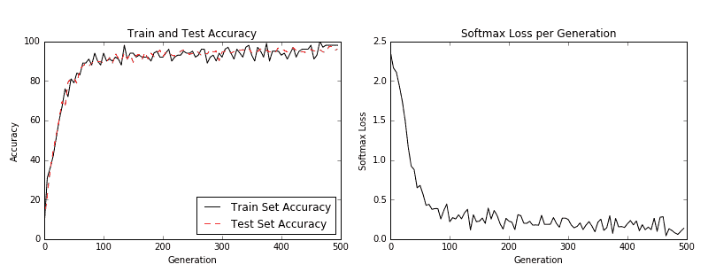圖 3：左圖是我們 500 代訓練中的訓練和測試集精度。右圖是超過 500 代的 softmax 損失值。 1. 如果我們想要繪制最新批次結果的樣本，下面是繪制由六個最新結果組成的樣本的代碼： ```py # Plot the 6 of the last batch results: actuals = rand_y[0:6] predictions = np.argmax(temp_train_preds,axis=1)[0:6] images = np.squeeze(rand_x[0:6]) Nrows = 2 Ncols = 3 for i in range(6): plt.subplot(Nrows, Ncols, i+1) plt.imshow(np.reshape(images[i], [28,28]), cmap='Greys_r') plt.title('Actual: ' + str(actuals[i]) + ' Pred: ' + str(predictions[i]), fontsize=10) frame = plt.gca() frame.axes.get_xaxis().set_visible(False) frame.axes.get_yaxis().set_visible(False) ``` 我們得到前面代碼的以下輸出：  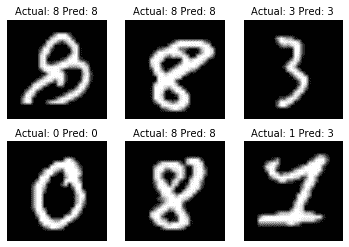圖 4：六個隨機圖像的繪圖，標題中包含實際值和預測值。右下圖預計是 3，而事實上它是 1 ## 工作原理 我們提高了 MNIST 數據集的表現，并構建了一個模型，在從頭開始訓練時，可快速達到約 97％的準確率。我們的前兩層是卷積，ReLU 和 Max Pooling 的組合。第二層是完全連接的層。我們以 100 個批次進行了訓練，并研究了我們訓練的幾代的準確率和損失。最后，我們還繪制了六個隨機數字和每個數字的預測/實際值。 CNN 非常適合圖像識別。造成這種情況的部分原因是卷積層創建了自己的低級特征，當它們遇到重要的部分圖像時會被激活。這種類型的模型自己創建特征并將其用于預測。 ## 更多 在過去幾年中，CNN 模型在圖像識別方面取得了巨大進步。正在探索許多新穎的想法，并且經常發現新的架構。該領域的一個很好的論文庫是一個名為 Arxiv.org（ [https://arxiv.org/](https://arxiv.org/) ）的倉庫網站，由康奈爾大學創建和維護。 Arxiv.org 包括許多領域的一些最新論文，包括計算機科學和計算機科學子領域，如計算機視覺和圖像識別（ [https://arxiv.org/list/cs.CV/recent](https://arxiv.org/list/cs.CV/recent) ）。 ## 另見 以下列出了一些可用于了解 CNN 的優秀資源： * 斯坦福大學有一個很棒的維基： [http://scarlet.stanford.edu/teach/index.php/An_Introduction_to_Convolutional_Neural_Networks](http://scarlet.stanford.edu/teach/index.php/An_Introduction_to_Convolutional_Neural_Networks) * 邁克爾·尼爾森的深度學習，在這里找到： [http://neuralnetworksanddeeplearning.com/chap6.html](http://neuralnetworksanddeeplearning.com/chap6.html) * 吳建新介紹卷積神經網絡，在此處找到： [https://pdfs.semanticscholar.org/450c/a19932fcef1ca6d0442cbf52fec38fb9d1e5.pdf](https://pdfs.semanticscholar.org/450c/a19932fcef1ca6d0442cbf52fec38fb9d1e5.pdf)