# 使用 k 均值聚類 TensorFlow 還可用于實現迭代聚類算法，例如 k-means。在本文中，我們展示了在`iris`數據集上使用 k-means 的示例。 ## 做好準備 我們在本書中探討的幾乎所有機器學習模型都是監督模型。 TensorFlow 非常適合這些類型的問題。但是，如果我們愿意，我們也可以實現無人監督的模型。例如，此秘籍將實現 k-means 聚類。 我們將實現聚類的數據集是`iris`數據集。這是一個很好的數據集的原因之一是因為我們已經知道有三種不同的目標（三種類型的鳶尾花）。這讓我們知道我們正在尋找數據中的三個不同的集群。 我們將`iris`數據集聚類為三組，然后將這些聚類的準確率與實際標簽進行比較。 ## 操作步驟 1. 首先，我們加載必要的庫。我們還從`sklearn`加載了一些 PCA 工具，以便我們可以將結果數據從四維更改為二維，以實現可視化目的： ```py import numpy as np import matplotlib.pyplot as plt import tensorflow as tf from sklearn import datasets from scipy.spatial import cKDTree from sklearn.decomposition import PCA from sklearn.preprocessing import scale ``` 1. 我們啟動圖會話，并加載`iris`數據集： ```py sess = tf.Session() iris = datasets.load_iris() num_pts = len(iris.data) num_feats = len(iris.data[0]) ``` 1. 我們現在將設置組，代，并創建圖所需的變量： ```py k=3 generations = 25 data_points = tf.Variable(iris.data) cluster_labels = tf.Variable(tf.zeros([num_pts], dtype=tf.int64)) ``` 1. 我們需要的下一個變量是每組的質心。我們將通過隨機選擇`iris`數據集的三個不同點來初始化 k-means 算法的質心： ```py rand_starts = np.array([iris.data[np.random.choice(len(iris.data))] for _ in range(k)]) centroids = tf.Variable(rand_starts) ``` 1. 現在，我們需要計算每個數據點和每個`centroids`之間的距離。我們通過將`centroids`擴展為矩陣來實現這一點，對數據點也是如此。然后我們將計算兩個矩陣之間的歐幾里德距離： ```py centroid_matrix = tf.reshape(tf.tile(centroids, [num_pts, 1]), [num_pts, k, num_feats]) point_matrix = tf.reshape(tf.tile(data_points, [1, k]), [num_pts, k, num_feats]) distances = tf.reduce_sum(tf.square(point_matrix - centroid_matrix), reduction_indices=2) ``` 1. `centroids`賦值是每個數據點最接近的`centroids`（最小距離）： ```py centroid_group = tf.argmin(distances, 1) ``` 1. 現在，我們必須計算組平均值以獲得新的質心： ```py def data_group_avg(group_ids, data): # Sum each group sum_total = tf.unsorted_segment_sum(data, group_ids, 3) # Count each group num_total = tf.unsorted_segment_sum(tf.ones_like(data), group_ids, 3) # Calculate average avg_by_group = sum_total/num_total return(avg_by_group) means = data_group_avg(centroid_group, data_points) update = tf.group(centroids.assign(means), cluster_labels.assign(centroid_group)) ``` 1. 接下來，我們初始化模型變量： ```py init = tf.global_variables_initializer() sess.run(init) ``` 1. 我們將遍歷幾代并相應地更新每個組的質心： ```py for i in range(generations): print('Calculating gen {}, out of {}.'.format(i, generations)) _, centroid_group_count = sess.run([update, centroid_group]) group_count = [] for ix in range(k): group_count.append(np.sum(centroid_group_count==ix)) print('Group counts: {}'.format(group_count)) ``` 1. 這導致以下輸出： ```py Calculating gen 0, out of 25\. Group counts: [50, 28, 72] Calculating gen 1, out of 25\. Group counts: [50, 35, 65] Calculating gen 23, out of 25\. Group counts: [50, 38, 62] Calculating gen 24, out of 25\. Group counts: [50, 38, 62] ``` 1. 為了驗證我們的聚類，我們可以使用聚類進行預測。我們現在看到有多少數據點位于相同虹膜種類的相似簇中： ```py [centers, assignments] = sess.run([centroids, cluster_labels]) def most_common(my_list): return(max(set(my_list), key=my_list.count)) label0 = most_common(list(assignments[0:50])) label1 = most_common(list(assignments[50:100])) label2 = most_common(list(assignments[100:150])) group0_count = np.sum(assignments[0:50]==label0) group1_count = np.sum(assignments[50:100]==label1) group2_count = np.sum(assignments[100:150]==label2) accuracy = (group0_count + group1_count + group2_count)/150\. print('Accuracy: {:.2}'.format(accuracy)) ``` 1. 這導致以下輸出： ```py Accuracy: 0.89 ``` 1. 為了直觀地看到我們的分組，如果它們確實已經分離出`iris`物種，我們將使用 PCA 將四維轉換為二維，并繪制數據點和組。在 PCA 分解之后，我們在 x-y 值網格上創建預測，以繪制顏色圖： ```py pca_model = PCA(n_components=2) reduced_data = pca_model.fit_transform(iris.data) # Transform centers reduced_centers = pca_model.transform(centers) # Step size of mesh for plotting h = .02 x_min, x_max = reduced_data[:, 0].min() - 1, reduced_data[:, 0].max() + 1 y_min, y_max = reduced_data[:, 1].min() - 1, reduced_data[:, 1].max() + 1 xx, yy = np.meshgrid(np.arange(x_min, x_max, h), np.arange(y_min, y_max, h)) # Get k-means classifications for the grid points xx_pt = list(xx.ravel()) yy_pt = list(yy.ravel()) xy_pts = np.array([[x,y] for x,y in zip(xx_pt, yy_pt)]) mytree = cKDTree(reduced_centers) dist, indexes = mytree.query(xy_pts) indexes = indexes.reshape(xx.shape) ``` 1. 并且，這里是`matplotlib`代碼將我們的發現結合在一個繪圖上。這個密碼的繪圖部分很大程度上改編自 scikit-learn（ [http://scikit-learn.org/](http://scikit-learn.org/) ）文檔網站上的演示（ [http://scikit-learn.org/ stable / auto_examples / cluster / plot_kmeans_digits.html](http://scikit-learn.org/stable/auto_examples/cluster/plot_kmeans_digits.html) ）： ```py plt.clf() plt.imshow(indexes, interpolation='nearest', extent=(xx.min(), xx.max(), yy.min(), yy.max()), cmap=plt.cm.Paired, aspect='auto', origin='lower') # Plot each of the true iris data groups symbols = ['o', '^', 'D'] label_name = ['Setosa', 'Versicolour', 'Virginica'] for i in range(3): temp_group = reduced_data[(i*50):(50)*(i+1)] plt.plot(temp_group[:, 0], temp_group[:, 1], symbols[i], markersize=10, label=label_name[i]) # Plot the centroids as a white X plt.scatter(reduced_centers[:, 0], reduced_centers[:, 1], marker='x', s=169, linewidths=3, color='w', zorder=10) plt.title('K-means clustering on Iris Datasets' 'Centroids are marked with white cross') plt.xlim(x_min, x_max) plt.ylim(y_min, y_max) plt.legend(loc='lower right') plt.show() ``` 這個繪圖代碼將向我們展示三個類，三個類的預測空間以及每個組的質心：  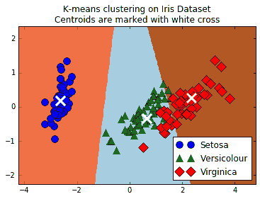圖 5：顯示 k-means 的無監督分類算法的屏幕截圖;可以用來將三種鳶尾花種組合在一起。三個 k-means 組是三個陰影區域，三個不同的點（圓，三角形和菱形）是三個真正的物種分類 ## 更多 對于此秘籍，我們使用 TensorFlow 將`iris`數據集聚類為三組。然后，我們計算了落入相似組的數據點的百分比（89％），并繪制了所得 k-均值組的圖。由于 k-means 作為分類算法是局部線性的（線性分離器向上），因此很難學習虹膜鳶尾和 Iris virginica 之間的天然非線性邊界。但是，一個優點是 k-means 算法根本不需要標記數據來執行。