# 實現非線性 SVM 對于此秘籍，我們將應用非線性內核來拆分數據集。 ## 做好準備 在本節中，我們將在實際數據上實現前面的高斯核 SVM。我們將加載虹膜數據集并為 I. setosa 創建分類器（與非 setosa 相比）。我們將看到各種伽馬值對分類的影響。 ## 操作步驟 我們按如下方式處理秘籍： 1. 我們首先加載必要的庫，其中包括`scikit-learn`數據集，以便我們可以加載虹膜數據。然后，我們將開始圖會話。使用以下代碼： ```py import matplotlib.pyplot as plt import numpy as np import tensorflow as tf from sklearn import datasets sess = tf.Session() ``` 1. 接下來，我們將加載虹膜數據，提取萼片長度和花瓣寬度，并分離每個類的`x`和`y`值（以便以后繪圖），如下所示： ```py iris = datasets.load_iris() x_vals = np.array([[x[0], x[3]] for x in iris.data]) y_vals = np.array([1 if y==0 else -1 for y in iris.target]) class1_x = [x[0] for i,x in enumerate(x_vals) if y_vals[i]==1] class1_y = [x[1] for i,x in enumerate(x_vals) if y_vals[i]==1] class2_x = [x[0] for i,x in enumerate(x_vals) if y_vals[i]==-1] class2_y = [x[1] for i,x in enumerate(x_vals) if y_vals[i]==-1] ``` 1. 現在，我們聲明我們的批量大小（首選大批量），占位符和模型變量`b`，如下所示： ```py batch_size = 100 x_data = tf.placeholder(shape=[None, 2], dtype=tf.float32) y_target = tf.placeholder(shape=[None, 1], dtype=tf.float32) prediction_grid = tf.placeholder(shape=[None, 2], dtype=tf.float32) b = tf.Variable(tf.random_normal(shape=[1,batch_size])) ``` 1. 接下來，我們聲明我們的高斯內核。這個內核依賴于伽馬值，我們將在本文后面的各個伽瑪值對分類的影響進行說明。使用以下代碼： ```py gamma = tf.constant(-10.0) dist = tf.reduce_sum(tf.square(x_data), 1) dist = tf.reshape(dist, [-1,1]) sq_dists = tf.add(tf.subtract(dist, tf.multiply(2., tf.matmul(x_data, tf.transpose(x_data)))), tf.transpose(dist)) my_kernel = tf.exp(tf.multiply(gamma, tf.abs(sq_dists))) # We now compute the loss for the dual optimization problem, as follows: model_output = tf.matmul(b, my_kernel) first_term = tf.reduce_sum(b) b_vec_cross = tf.matmul(tf.transpose(b), b) y_target_cross = tf.matmul(y_target, tf.transpose(y_target)) second_term = tf.reduce_sum(tf.multiply(my_kernel, tf.multiply(b_vec_cross, y_target_cross))) loss = tf.negative(tf.subtract(first_term, second_term)) ``` 1. 為了使用 SVM 執行預測，我們必須創建預測內核函數。之后，我們還會聲明一個準確率計算，它只是使用以下代碼正確分類的點的百分比： ```py rA = tf.reshape(tf.reduce_sum(tf.square(x_data), 1),[-1,1]) rB = tf.reshape(tf.reduce_sum(tf.square(prediction_grid), 1),[-1,1]) pred_sq_dist = tf.add(tf.subtract(rA, tf.mul(2., tf.matmul(x_data, tf.transpose(prediction_grid)))), tf.transpose(rB)) pred_kernel = tf.exp(tf.multiply(gamma, tf.abs(pred_sq_dist))) prediction_output = tf.matmul(tf.multiply(tf.transpose(y_target),b), pred_kernel) prediction = tf.sign(prediction_output-tf.reduce_mean(prediction_output)) accuracy = tf.reduce_mean(tf.cast(tf.equal(tf.squeeze(prediction), tf.squeeze(y_target)), tf.float32)) ``` 1. 接下來，我們聲明我們的優化函數并初始化變量，如下所示： ```py my_opt = tf.train.GradientDescentOptimizer(0.01) train_step = my_opt.minimize(loss) init = tf.initialize_all_variables() sess.run(init) ``` 1. 現在，我們可以開始訓練循環了。我們運行循環 300 次迭代并存儲損失值和批次精度。為此，我們使用以下實現： ```py loss_vec = [] batch_accuracy = [] for i in range(300): rand_index = np.random.choice(len(x_vals), size=batch_size) rand_x = x_vals[rand_index] rand_y = np.transpose([y_vals[rand_index]]) sess.run(train_step, feed_dict={x_data: rand_x, y_target: rand_y}) temp_loss = sess.run(loss, feed_dict={x_data: rand_x, y_target: rand_y}) loss_vec.append(temp_loss) acc_temp = sess.run(accuracy, feed_dict={x_data: rand_x, y_target: rand_y, prediction_grid:rand_x}) batch_accuracy.append(acc_temp) ``` 1. 為了繪制決策邊界，我們將創建`x`，`y`點的網格并評估我們在所有這些點上創建的預測函數，如下所示： ```py x_min, x_max = x_vals[:, 0].min() - 1, x_vals[:, 0].max() + 1 y_min, y_max = x_vals[:, 1].min() - 1, x_vals[:, 1].max() + 1 xx, yy = np.meshgrid(np.arange(x_min, x_max, 0.02), np.arange(y_min, y_max, 0.02)) grid_points = np.c_[xx.ravel(), yy.ravel()] [grid_predictions] = sess.run(prediction, feed_dict={x_data: x_vals, y_target: np.transpose([y_vals]), prediction_grid: grid_points}) grid_predictions = grid_predictions.reshape(xx.shape) ``` 1. 為簡潔起見，我們只展示如何用決策邊界繪制點。有關 gamma 的圖和效果，請參閱本秘籍的下一部分。使用以下代碼： ```py plt.contourf(xx, yy, grid_predictions, cmap=plt.cm.Paired, alpha=0.8) plt.plot(class1_x, class1_y, 'ro', label='I. setosa') plt.plot(class2_x, class2_y, 'kx', label='Non-setosa') plt.title('Gaussian SVM Results on Iris Data') plt.xlabel('Petal Length') plt.ylabel('Sepal Width') plt.legend(loc='lower right') plt.ylim([-0.5, 3.0]) plt.xlim([3.5, 8.5]) plt.show() ``` ## 工作原理 以下是對四種不同伽瑪值（1,10,25 和 100）的 I. setosa 結果的分類。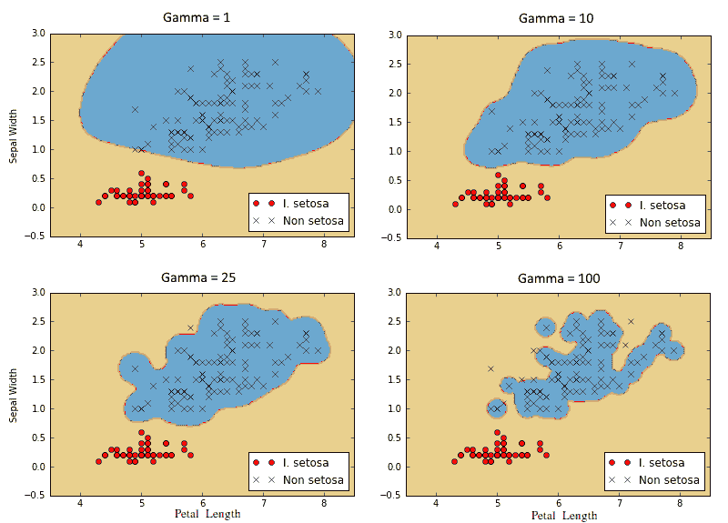注意伽瑪值越高，每個單獨點對分類邊界的影響越大：  圖 9：使用具有四個不同伽馬值的高斯核 SVM 的 I. setosa 的分類結果