如何開發單變量時間序列預測的深度學習模型 · Machine Learning Mastery 博客文章翻譯

# 如何開發單變量時間序列預測的深度學習模型 > 原文： [https://machinelearningmastery.com/how-to-develop-deep-learning-models-for-univariate-time-series-forecasting/](https://machinelearningmastery.com/how-to-develop-deep-learning-models-for-univariate-time-series-forecasting/) 深度學習神經網絡能夠自動學習和從原始數據中提取特征。神經網絡的這一特征可用于時間序列預測問題，其中模型可以直接在原始觀測上開發，而不需要使用歸一化和標準化來擴展數據或通過差分使數據靜止。令人印象深刻的是，簡單的深度學習神經網絡模型能夠進行熟練的預測，與樸素模型和調整 SARIMA 模型相比，單變量時間序列預測存在趨勢和季節性成分且無需預處理的問題。在本教程中，您將了解如何開發一套用于單變量時間序列預測的深度學習模型。完成本教程后，您將了解： * 如何使用前向驗證開發一個強大的測試工具來評估神經網絡模型的表現。 * 如何開發和評估簡單多層感知器和卷積神經網絡的時間序列預測。 * 如何開發和評估 LSTM，CNN-LSTM 和 ConvLSTM 神經網絡模型用于時間序列預測。讓我們開始吧。 ![How to Develop Deep Learning Models for Univariate Time Series Forecasting](https://img.kancloud.cn/79/a6/79a64b43dbf2aed03ffcbb82791087d8_640x277.jpg) 如何開發單變量時間序列預測的深度學習模型照片由 [Nathaniel McQueen](https://www.flickr.com/photos/nmcqueenphotography/40518405705/) ，保留一些權利。 ## 教程概述本教程分為五個部分;他們是： 1. 問題描述 2. 模型評估測試線束 3. 多層感知器模型 4. 卷積神經網絡模型 5. 循環神經網絡模型 ## 問題描述 '_ 月度汽車銷售 _'數據集總結了 1960 年至 1968 年間加拿大魁北克省的月度汽車銷量。您可以從 [DataMarket](https://datamarket.com/data/set/22n4/monthly-car-sales-in-quebec-1960-1968#!ds=22n4&display=line) 了解有關數據集的更多信息。直接從這里下載數據集： * [month-car-sales.csv](https://raw.githubusercontent.com/jbrownlee/Datasets/master/monthly-car-sales.csv) 在當前工作目錄中使用文件名“ _monthly-car-sales.csv_ ”保存文件。我們可以使用函數 _read_csv（）_ 將此數據集作為 Pandas 系列加載。 ```py # load series = read_csv('monthly-car-sales.csv', header=0, index_col=0) ``` 加載后，我們可以總結數據集的形狀，以確定觀察的數量。 ```py # summarize shape print(series.shape) ``` 然后我們可以創建該系列的線圖，以了解該系列的結構。 ```py # plot pyplot.plot(series) pyplot.show() ``` 我們可以將所有這些結合在一起;下面列出了完整的示例。 ```py # load and plot dataset from pandas import read_csv from matplotlib import pyplot # load series = read_csv('monthly-car-sales.csv', header=0, index_col=0) # summarize shape print(series.shape) # plot pyplot.plot(series) pyplot.show() ``` 首先運行該示例將打印數據集的形狀。 ```py (108, 1) ``` 該數據集是每月一次，有 9 年或 108 次觀測。在我們的測試中，將使用去年或 12 個觀測值作為測試集。創建線圖。數據集具有明顯的趨勢和季節性成分。季節性成分的期限可能是六個月或 12 個月。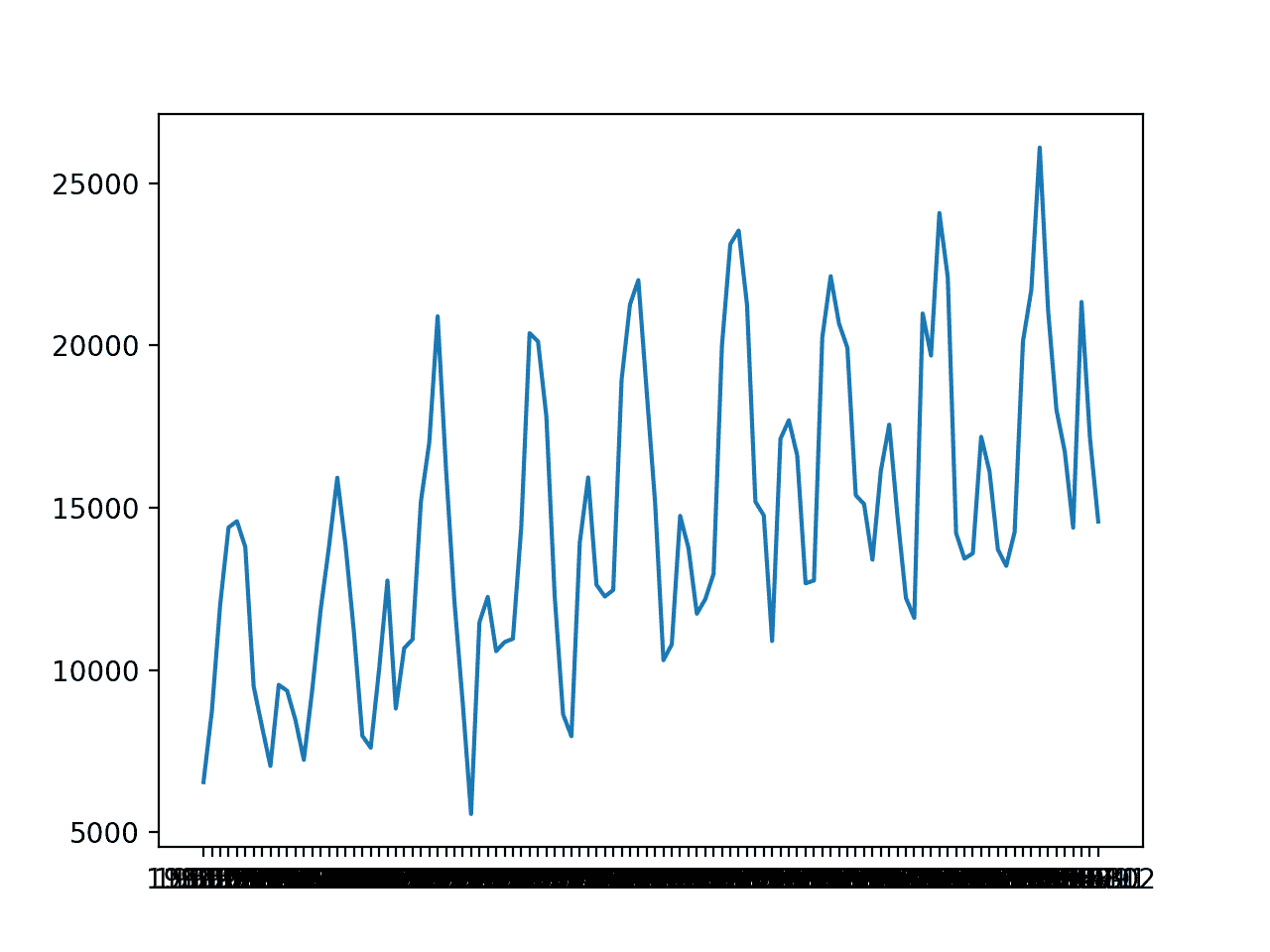 ![Line Plot of Monthly Car Sales](https://img.kancloud.cn/79/4e/794e2be5483d741bc2f967eb2e8b9722_1280x960.jpg) 月度汽車銷售線圖從之前的實驗中，我們知道一個幼稚的模型可以通過取預測月份的前三年的觀測值的中位數來實現 1841.155 的均方根誤差或 RMSE;例如： ```py yhat = median(-12, -24, -36) ``` 負指數是指相對于預測月份的歷史數據末尾的序列中的觀察值。從之前的實驗中，我們知道 SARIMA 模型可以達到 1551.842 的 RMSE，其配置為 SARIMA（0,0,0），（1,1,0），12 其中沒有為趨勢指定元素和季節性差異計算周期為 12，并使用一個季節的 AR 模型。樸素模型的表現為被認為熟練的模型提供了下限。任何在過去 12 個月內達到低于 1841.155 的預測表現的模型都具有技巧。 SARIMA 模型的表現可以衡量問題的良好模型。任何在過去 12 個月內達到預測表現低于 1551.842 的模型都應采用 SARIMA 模型。現在我們已經定義了模型技能的問題和期望，我們可以看看定義測試工具。 ## 模型評估測試線束在本節中，我們將開發一個測試工具，用于開發和評估不同類型的神經網絡模型，用于單變量時間序列預測。本節分為以下幾部分： 1. 訓練 - 測試分裂 2. 系列作為監督學習 3. 前瞻性驗證 4. 重復評估 5. 總結表現 6. 工作示例 ### 訓練 - 測試分裂第一步是將加載的系列分成訓練和測試集。我們將使用前八年（96 個觀測值）進行訓練，最后 12 個用于測試集。下面的 _train_test_split（）_ 函數將拆分系列，將原始觀察值和在測試集中使用的觀察數作為參數。 ```py # split a univariate dataset into train/test sets def train_test_split(data, n_test): return data[:-n_test], data[-n_test:] ``` ### 系列作為監督學習接下來，我們需要能夠將單變量觀測系列框架化為監督學習問題，以便我們可以訓練神經網絡模型。系列的監督學習框架意味著需要將數據拆分為模型從中學習和概括的多個示例。每個樣本必須同時具有輸入組件和輸出組件。輸入組件將是一些先前的觀察，例如三年或 36 個時間步驟。輸出組件將是下個月的總銷售額，因為我們有興趣開發一個模型來進行一步預測。我們可以使用 pandas DataFrame 上的 [shift（）函數](http://pandas-docs.github.io/pandas-docs-travis/generated/pandas.DataFrame.shift.html)來實現它。它允許我們向下移動一列（向前移動）或向后移動（向后移動）。我們可以將該系列作為一列數據，然后創建列的多個副本，向前或向后移動，以便使用我們需要的輸入和輸出元素創建樣本。當一個系列向下移動時，會引入 _NaN_ 值，因為我們沒有超出系列開頭的值。例如，系列定義為列： ```py (t) 1 2 3 4 ``` 可以預先移位和插入列： ```py (t-1), (t) Nan, 1 1, 2 2, 3 3, 4 4 NaN ``` 我們可以看到，在第二行，值 1 作為輸入提供，作為前一時間步的觀察，2 是系列中可以預測的下一個值，或者當 1 是預測模型時要學習的值作為輸入呈現。可以去除具有 _NaN_ 值的行。下面的 _series_to_supervised（）_ 函數實現了這種行為，允許您指定輸入中使用的滯后觀察數和每個樣本的輸出中使用的數。它還將刪除具有 _NaN_ 值的行，因為它們不能用于訓練或測試模型。 ```py # transform list into supervised learning format def series_to_supervised(data, n_in=1, n_out=1): df = DataFrame(data) cols = list() # input sequence (t-n, ... t-1) for i in range(n_in, 0, -1): cols.append(df.shift(i)) # forecast sequence (t, t+1, ... t+n) for i in range(0, n_out): cols.append(df.shift(-i)) # put it all together agg = concat(cols, axis=1) # drop rows with NaN values agg.dropna(inplace=True) return agg.values ``` ### 前瞻性驗證可以使用[前進驗證](https://machinelearningmastery.com/backtest-machine-learning-models-time-series-forecasting/)在測試集上評估時間序列預測模型。前瞻性驗證是一種方法，其中模型一次一個地對測試數據集中的每個觀察進行預測。在對測試數據集中的時間步長進行每個預測之后，將預測的真實觀察結果添加到測試數據集并使其可用于模型。在進行后續預測之前，可以使用觀察結果更簡單的模型。考慮到更高的計算成本，更復雜的模型，例如神經網絡，不會被改裝。然而，時間步驟的真實觀察可以用作輸入的一部分，用于在下一個時間步驟上進行預測。首先，數據集分為訓練集和測試集。我們將調用 _train_test_split（）_ 函數來執行此拆分并傳入預先指定數量的觀察值以用作測試數據。對于給定配置，模型將適合訓練數據集一次。我們將定義一個通用的 _model_fit（）_ 函數來執行此操作，可以為我們稍后可能感興趣的給定類型的神經網絡填充該操作。該函數獲取訓練數據集和模型配置，并返回準備好進行預測的擬合模型。 ```py # fit a model def model_fit(train, config): return None ``` 枚舉測試數據集的每個時間步。使用擬合模型進行預測。同樣，我們將定義一個名為 _model_predict（）_ 的通用函數，它采用擬合模型，歷史和模型配置，并進行單個一步預測。 ```py # forecast with a pre-fit model def model_predict(model, history, config): return 0.0 ``` 將預測添加到預測列表中，并將來自測試集的真實觀察結果添加到用訓練數據集中的所有觀察結果播種的觀察列表中。此列表在前向驗證的每個步驟中構建，允許模型使用最新歷史記錄進行一步預測。然后可以將所有預測與測試集中的真實值進行比較，并計算誤差測量值。我們將計算預測和真實值之間的均方根誤差或 RMSE。 RMSE 計算為預測值與實際值之間的平方差的平均值的平方根。 _measure_rmse（）_ 使用 [mean_squared_error（）scikit-learn 函數](http://scikit-learn.org/stable/modules/generated/sklearn.metrics.mean_squared_error.html)在計算平方根之前首先計算均方誤差或 MSE。 ```py # root mean squared error or rmse def measure_rmse(actual, predicted): return sqrt(mean_squared_error(actual, predicted)) ``` 下面列出了將所有這些聯系在一起的完整 _walk_forward_validation（）_ 函數。它采用數據集，用作測試集的觀察數量以及模型的配置，并返回測試集上模型表現的 RMSE。 ```py # walk-forward validation for univariate data def walk_forward_validation(data, n_test, cfg): predictions = list() # split dataset train, test = train_test_split(data, n_test) # fit model model = model_fit(train, cfg) # seed history with training dataset history = [x for x in train] # step over each time-step in the test set for i in range(len(test)): # fit model and make forecast for history yhat = model_predict(model, history, cfg) # store forecast in list of predictions predictions.append(yhat) # add actual observation to history for the next loop history.append(test[i]) # estimate prediction error error = measure_rmse(test, predictions) print(' > %.3f' % error) return error ``` ### 重復評估神經網絡模型是隨機的。這意味著，在給定相同的模型配置和相同的訓練數據集的情況下，每次訓練模型時將產生不同的內部權重集，這反過來將具有不同的表現。這是一個好處，允許模型自適應并找到復雜問題的高表現配置。在評估模型的表現和選擇用于進行預測的最終模型時，這也是一個問題。為了解決模型評估問題，我們將通過前向驗證多次評估模型配置，并將錯誤報告為每次評估的平均誤差。對于大型神經網絡而言，這并不總是可行的，并且可能僅適用于能夠在幾分鐘或幾小時內完成的小型網絡。下面的 _repeat_evaluate（）_ 函數實現了這一點，并允許將重復次數指定為默認為 30 的可選參數，并返回模型表現得分列表：在本例中為 RMSE 值。 ```py # repeat evaluation of a config def repeat_evaluate(data, config, n_test, n_repeats=30): # fit and evaluate the model n times scores = [walk_forward_validation(data, n_test, config) for _ in range(n_repeats)] return scores ``` ### 總結表現最后，我們需要從多個重復中總結模型的表現。我們將首先使用匯總統計匯總表現，特別是平均值和標準差。我們還將使用盒子和須狀圖繪制模型表現分數的分布，以幫助了解表現的傳播。下面的 _summarize_scores（）_ 函數實現了這一點，取了評估模型的名稱和每次重復評估的分數列表，打印摘要并顯示圖表。 ```py # summarize model performance def summarize_scores(name, scores): # print a summary scores_m, score_std = mean(scores), std(scores) print('%s: %.3f RMSE (+/- %.3f)' % (name, scores_m, score_std)) # box and whisker plot pyplot.boxplot(scores) pyplot.show() ``` ### 工作示例現在我們已經定義了測試工具的元素，我們可以將它們綁定在一起并定義一個簡單的持久性模型。具體而言，我們將計算先前觀察的子集相對于預測時間的中值。我們不需要擬合模型，因此 _model_fit（）_ 函數將被實現為簡單地返回 _ 無 _。 ```py # fit a model def model_fit(train, config): return None ``` 我們將使用配置來定義先前觀察中的索引偏移列表，該列表相對于將被用作預測的預測時間。例如，12 將使用 12 個月前（-12）相對于預測時間的觀察。 ```py # define config config = [12, 24, 36] ``` 可以實現 model_predict（）函數以使用此配置來收集觀察值，然后返回這些觀察值的中值。 ```py # forecast with a pre-fit model def model_predict(model, history, config): values = list() for offset in config: values.append(history[-offset]) return median(values) ``` 下面列出了使用簡單持久性模型使用框架的完整示例。 ```py # persistence from math import sqrt from numpy import mean from numpy import std from pandas import DataFrame from pandas import concat from pandas import read_csv from sklearn.metrics import mean_squared_error from matplotlib import pyplot # split a univariate dataset into train/test sets def train_test_split(data, n_test): return data[:-n_test], data[-n_test:] # transform list into supervised learning format def series_to_supervised(data, n_in=1, n_out=1): df = DataFrame(data) cols = list() # input sequence (t-n, ... t-1) for i in range(n_in, 0, -1): cols.append(df.shift(i)) # forecast sequence (t, t+1, ... t+n) for i in range(0, n_out): cols.append(df.shift(-i)) # put it all together agg = concat(cols, axis=1) # drop rows with NaN values agg.dropna(inplace=True) return agg.values # root mean squared error or rmse def measure_rmse(actual, predicted): return sqrt(mean_squared_error(actual, predicted)) # difference dataset def difference(data, interval): return [data[i] - data[i - interval] for i in range(interval, len(data))] # fit a model def model_fit(train, config): return None # forecast with a pre-fit model def model_predict(model, history, config): values = list() for offset in config: values.append(history[-offset]) return median(values) # walk-forward validation for univariate data def walk_forward_validation(data, n_test, cfg): predictions = list() # split dataset train, test = train_test_split(data, n_test) # fit model model = model_fit(train, cfg) # seed history with training dataset history = [x for x in train] # step over each time-step in the test set for i in range(len(test)): # fit model and make forecast for history yhat = model_predict(model, history, cfg) # store forecast in list of predictions predictions.append(yhat) # add actual observation to history for the next loop history.append(test[i]) # estimate prediction error error = measure_rmse(test, predictions) print(' > %.3f' % error) return error # repeat evaluation of a config def repeat_evaluate(data, config, n_test, n_repeats=30): # fit and evaluate the model n times scores = [walk_forward_validation(data, n_test, config) for _ in range(n_repeats)] return scores # summarize model performance def summarize_scores(name, scores): # print a summary scores_m, score_std = mean(scores), std(scores) print('%s: %.3f RMSE (+/- %.3f)' % (name, scores_m, score_std)) # box and whisker plot pyplot.boxplot(scores) pyplot.show() series = read_csv('monthly-car-sales.csv', header=0, index_col=0) data = series.values # data split n_test = 12 # define config config = [12, 24, 36] # grid search scores = repeat_evaluate(data, config, n_test) # summarize scores summarize_scores('persistence', scores) ``` 運行該示例將打印在最近 12 個月的數據中使用前向驗證評估的模型的 RMSE。該模型被評估 30 次，但由于該模型沒有隨機元素，因此每次得分相同。 ```py > 1841.156 > 1841.156 > 1841.156 > 1841.156 > 1841.156 > 1841.156 > 1841.156 > 1841.156 > 1841.156 > 1841.156 > 1841.156 > 1841.156 > 1841.156 > 1841.156 > 1841.156 > 1841.156 > 1841.156 > 1841.156 > 1841.156 > 1841.156 > 1841.156 > 1841.156 > 1841.156 > 1841.156 > 1841.156 > 1841.156 > 1841.156 > 1841.156 > 1841.156 > 1841.156 persistence: 1841.156 RMSE (+/- 0.000) ``` 我們可以看到模型的 RMSE 是 1841，提供了表現的下限，通過它我們可以評估模型是否熟練掌握問題。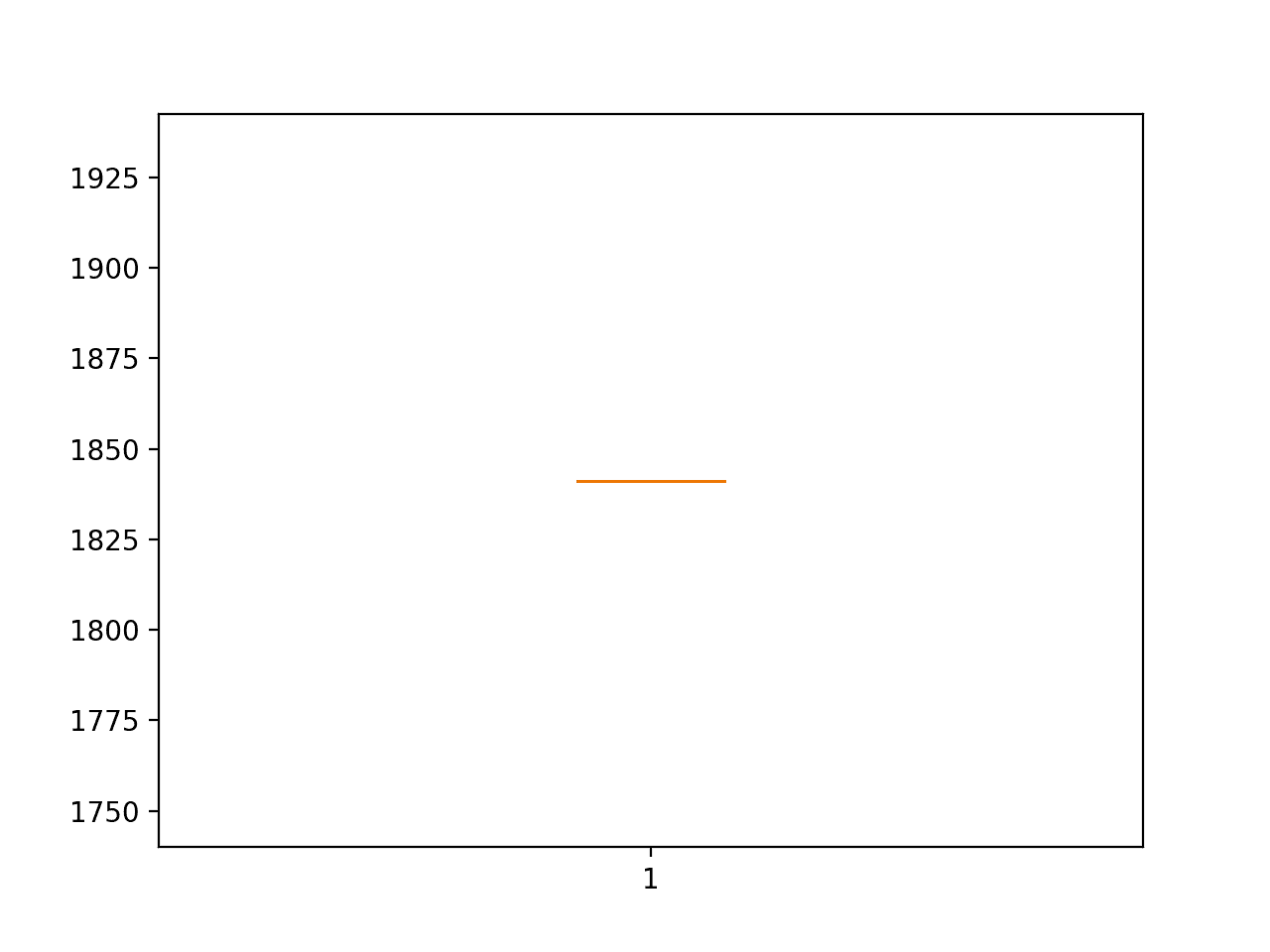 ![Box and Whisker Plot of Persistence RMSE Forecasting Car Sales](https://img.kancloud.cn/d4/e1/d4e126114218898e9a884b734ae36dce_1280x960.jpg) 持久性 RMSE 預測汽車銷售的盒子和晶須圖既然我們擁有強大的測試工具，我們就可以用它來評估一套神經網絡模型。 ## 多層感知器模型我們將評估的第一個網絡是多層感知器，簡稱 MLP。這是一個簡單的前饋神經網絡模型，應該在考慮更復雜的模型之前進行評估。 MLP 可用于時間序列預測，方法是在先前時間步驟中進行多次觀測，稱為滯后觀測，并將其用作輸入要素并根據這些觀測預測一個或多個時間步長。這正是上一節中 _series_to_supervised（）_ 函數提供的問題的框架。因此，訓練數據集是樣本列表，其中每個樣本在預測時間之前的幾個月具有一定數量的觀察，并且預測是序列中的下個月。例如： ```py X, y month1, month2, month3, month4 month2, month3, month4, month5 month3, month4, month5, month6 ... ``` 該模型將嘗試概括這些樣本，以便當提供超出模型已知的新樣本時，它可以預測有用的東西;例如： ```py X, y month4, month5, month6, ??? ``` 我們將使用 Keras 深度學習庫實現一個簡單的 MLP。該模型將具有輸入層，其具有一些先前的觀察結果。當我們定義第一個隱藏層時，可以使用 _input_dim_ 參數指定。該模型將具有單個隱藏層，其具有一定數量的節點，然后是單個輸出層。我們將在隱藏層上使用經過校正的線性激活函數，因為它表現良好。我們將在輸出層使用線性激活函數（默認值），因為我們正在預測連續值。網絡的損失函數將是均方誤差損失或 MSE，我們將使用隨機梯度下降的高效 [Adam 風格來訓練網絡。](https://machinelearningmastery.com/adam-optimization-algorithm-for-deep-learning/) ```py # define model model = Sequential() model.add(Dense(n_nodes, activation='relu', input_dim=n_input)) model.add(Dense(1)) model.compile(loss='mse', optimizer='adam') ``` 該模型將適合一些訓練時期（對訓練數據的暴露），并且可以指定批量大小以定義在每個時期內權重的更新頻率。下面列出了用于在訓練數據集上擬合 MLP 模型的 _model_fit（）_ 函數。該函數要求配置為具有以下配置超參數的列表： * **n_input** ：用作模型輸入的滯后觀察數。 * **n_nodes** ：隱藏層中使用的節點數。 * **n_epochs** ：將模型公開給整個訓練數據集的次數。 * **n_batch** ：更新權重的時期內的樣本數。 ```py # fit a model def model_fit(train, config): # unpack config n_input, n_nodes, n_epochs, n_batch = config # prepare data data = series_to_supervised(train, n_in=n_input) train_x, train_y = data[:, :-1], data[:, -1] # define model model = Sequential() model.add(Dense(n_nodes, activation='relu', input_dim=n_input)) model.add(Dense(1)) model.compile(loss='mse', optimizer='adam') # fit model.fit(train_x, train_y, epochs=n_epochs, batch_size=n_batch, verbose=0) return model ``` 使用擬合 MLP 模型進行預測與調用 _predict（）_ 函數并傳入進行預測所需的一個樣本值輸入值一樣簡單。 ```py yhat = model.predict(x_input, verbose=0) ``` 為了使預測超出已知數據的限制，這要求將最后 n 個已知觀察值作為數組并用作輸入。 _predict（）_ 函數在進行預測時需要一個或多個輸入樣本，因此提供單個樣本需要陣列具有[ _1，n_input_ ]形狀??，其中 _] n_input_ 是模型期望作為輸入的時間步數。類似地， _predict（）_ 函數返回一個預測數組，每個樣本一個作為輸入提供。在一個預測的情況下，將存在具有一個值的數組。下面的 _model_predict（）_ 函數實現了這種行為，將模型，先前觀察和模型配置作為參數，制定輸入樣本并進行一步預測，然后返回。 ```py # forecast with a pre-fit model def model_predict(model, history, config): # unpack config n_input, _, _, _ = config # prepare data x_input = array(history[-n_input:]).reshape(1, n_input) # forecast yhat = model.predict(x_input, verbose=0) return yhat[0] ``` 我們現在擁有在月度汽車銷售數據集上評估 MLP 模型所需的一切。進行模型超參數的簡單網格搜索，并選擇下面的配置。這可能不是最佳配置，但卻是最好的配置。 * **n_input** ：24（例如 24 個月） * **n_nodes** ：500 * **n_epochs** ：100 * **n_batch** ：100 此配置可以定義為列表： ```py # define config config = [24, 500, 100, 100] ``` 請注意，當訓練數據被構建為監督學習問題時，只有 72 個樣本可用于訓練模型。使用 72 或更大的批量大小意味著使用批量梯度下降而不是小批量梯度下降來訓練模型。這通常用于小數據集，并且意味著在每個時期結束時執行權重更新和梯度計算，而不是在每個時期內多次執行。完整的代碼示例如下所示。 ```py # evaluate mlp from math import sqrt from numpy import array from numpy import mean from numpy import std from pandas import DataFrame from pandas import concat from pandas import read_csv from sklearn.metrics import mean_squared_error from keras.models import Sequential from keras.layers import Dense from matplotlib import pyplot # split a univariate dataset into train/test sets def train_test_split(data, n_test): return data[:-n_test], data[-n_test:] # transform list into supervised learning format def series_to_supervised(data, n_in=1, n_out=1): df = DataFrame(data) cols = list() # input sequence (t-n, ... t-1) for i in range(n_in, 0, -1): cols.append(df.shift(i)) # forecast sequence (t, t+1, ... t+n) for i in range(0, n_out): cols.append(df.shift(-i)) # put it all together agg = concat(cols, axis=1) # drop rows with NaN values agg.dropna(inplace=True) return agg.values # root mean squared error or rmse def measure_rmse(actual, predicted): return sqrt(mean_squared_error(actual, predicted)) # fit a model def model_fit(train, config): # unpack config n_input, n_nodes, n_epochs, n_batch = config # prepare data data = series_to_supervised(train, n_in=n_input) train_x, train_y = data[:, :-1], data[:, -1] # define model model = Sequential() model.add(Dense(n_nodes, activation='relu', input_dim=n_input)) model.add(Dense(1)) model.compile(loss='mse', optimizer='adam') # fit model.fit(train_x, train_y, epochs=n_epochs, batch_size=n_batch, verbose=0) return model # forecast with a pre-fit model def model_predict(model, history, config): # unpack config n_input, _, _, _ = config # prepare data x_input = array(history[-n_input:]).reshape(1, n_input) # forecast yhat = model.predict(x_input, verbose=0) return yhat[0] # walk-forward validation for univariate data def walk_forward_validation(data, n_test, cfg): predictions = list() # split dataset train, test = train_test_split(data, n_test) # fit model model = model_fit(train, cfg) # seed history with training dataset history = [x for x in train] # step over each time-step in the test set for i in range(len(test)): # fit model and make forecast for history yhat = model_predict(model, history, cfg) # store forecast in list of predictions predictions.append(yhat) # add actual observation to history for the next loop history.append(test[i]) # estimate prediction error error = measure_rmse(test, predictions) print(' > %.3f' % error) return error # repeat evaluation of a config def repeat_evaluate(data, config, n_test, n_repeats=30): # fit and evaluate the model n times scores = [walk_forward_validation(data, n_test, config) for _ in range(n_repeats)] return scores # summarize model performance def summarize_scores(name, scores): # print a summary scores_m, score_std = mean(scores), std(scores) print('%s: %.3f RMSE (+/- %.3f)' % (name, scores_m, score_std)) # box and whisker plot pyplot.boxplot(scores) pyplot.show() series = read_csv('monthly-car-sales.csv', header=0, index_col=0) data = series.values # data split n_test = 12 # define config config = [24, 500, 100, 100] # grid search scores = repeat_evaluate(data, config, n_test) # summarize scores summarize_scores('mlp', scores) ``` 運行該示例為模型的 30 次重復評估中的每一次打印 RMSE。在運行結束時，報告的平均和標準偏差 RMSE 約為 1,526 銷售。我們可以看到，平均而言，所選配置的表現優于樸素模型（1841.155）和 SARIMA 模型（1551.842）。這是令人印象深刻的，因為該模型直接對原始數據進行操作而不進行縮放或數據靜止。 ```py > 1629.203 > 1642.219 > 1472.483 > 1662.055 > 1452.480 > 1465.535 > 1116.253 > 1682.667 > 1642.626 > 1700.183 > 1444.481 > 1673.217 > 1602.342 > 1655.895 > 1319.387 > 1591.972 > 1592.574 > 1361.607 > 1450.348 > 1314.529 > 1549.505 > 1569.750 > 1427.897 > 1478.926 > 1474.990 > 1458.993 > 1643.383 > 1457.925 > 1558.934 > 1708.278 mlp: 1526.688 RMSE (+/- 134.789) ``` 創建 RMSE 分數的方框和胡須圖，以總結模型表現的傳播。這有助于理解分數的傳播。我們可以看到，盡管平均而言模型的表現令人印象深刻，但傳播幅度很大。標準偏差略大于 134 銷售額，這意味著更糟糕的案例模型運行，誤差與平均誤差相差 2 或 3 個標準差可能比樸素模型差。使用 MLP 模型的一個挑戰是如何利用更高的技能并在多次運行中最小化模型的方差。該問題通常適用于神經網絡。您可以使用許多策略，但最簡單的方法可能就是在所有可用數據上訓練多個最終模型，并在進行預測時在集合中使用它們，例如：預測是 10 到 30 個模型的平均值。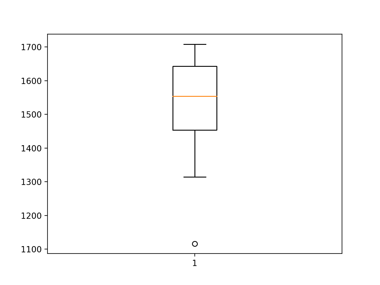 ![Box and Whisker Plot of Multilayer Perceptron RMSE Forecasting Car Sales](https://img.kancloud.cn/27/aa/27aa1b2ac190be534d507a8f7b5f9351_1280x960.jpg) 多層感知器 RMSE 預測汽車銷售的盒子和晶須圖 ## 卷積神經網絡模型卷積神經網絡（CNN）是為二維圖像數據開發的一種神經網絡，盡管它們可用于一維數據，例如文本序列和時間序列。當對一維數據進行操作時，CNN 讀取一系列滯后觀察并學習提取與進行預測相關的特征。我們將定義具有兩個卷積層的 CNN，用于從輸入序列中提取特征。每個都將具有可配置數量的濾波器和內核大小，并將使用經過整流的線性激活功能。濾波器的數量決定了讀取和投影加權輸入的并行字段的數量。內核大小定義了網絡沿輸入序列讀取時每個快照內讀取的時間步數。 ```py model.add(Conv1D(filters=n_filters, kernel_size=n_kernel, activation='relu', input_shape=(n_input, 1))) model.add(Conv1D(filters=n_filters, kernel_size=n_kernel, activation='relu')) ``` 在卷積層之后使用最大池化層將加權輸入特征提取為最顯著的特征，將輸入大小減小 1/4。匯總輸入在被解釋之前被平展為一個長向量，并用于進行一步預測。 ```py model.add(MaxPooling1D(pool_size=2)) model.add(Flatten()) model.add(Dense(1)) ``` CNN 模型期望輸入數據采用多個樣本的形式，其中每個樣本具有多個輸入時間步長，與上一節中的 MLP 相同。一個區別是 CNN 可以在每個時間步驟支持多個特征或類型的觀察，其被解釋為圖像的通道。我們在每個時間步都只有一個特征，因此輸入數據所需的三維形狀將是[ _n_samples，n_input，1_ ]。 ```py train_x = train_x.reshape((train_x.shape[0], train_x.shape[1], 1)) ``` 下面列出了用于在訓練數據集上擬合 CNN 模型的 _model_fit（）_ 函數。該模型將以下五個配置參數作為列表： * **n_input** ：用作模型輸入的滯后觀察數。 * **n_filters** ：并行濾波器的數量。 * **n_kernel** ：每次讀取輸入序列時考慮的時間步數。 * **n_epochs** ：將模型公開給整個訓練數據集的次數。 * **n_batch** ：更新權重的時期內的樣本數。 ```py # fit a model def model_fit(train, config): # unpack config n_input, n_filters, n_kernel, n_epochs, n_batch = config # prepare data data = series_to_supervised(train, n_in=n_input) train_x, train_y = data[:, :-1], data[:, -1] train_x = train_x.reshape((train_x.shape[0], train_x.shape[1], 1)) # define model model = Sequential() model.add(Conv1D(filters=n_filters, kernel_size=n_kernel, activation='relu', input_shape=(n_input, 1))) model.add(Conv1D(filters=n_filters, kernel_size=n_kernel, activation='relu')) model.add(MaxPooling1D(pool_size=2)) model.add(Flatten()) model.add(Dense(1)) model.compile(loss='mse', optimizer='adam') # fit model.fit(train_x, train_y, epochs=n_epochs, batch_size=n_batch, verbose=0) return model ``` 使用擬合 CNN 模型進行預測非常類似于使用上一節中的擬合 MLP 模型進行預測。一個區別在于我們要求我們指定在每個時間步驟觀察到的特征數量，在這種情況下為 1.因此，當進行單個一步預測時，輸入數組的形狀必須是： ```py [1, n_input, 1] ``` 下面的 _model_predict（）_ 函數實現了這種行為。 ```py # forecast with a pre-fit model def model_predict(model, history, config): # unpack config n_input, _, _, _, _ = config # prepare data x_input = array(history[-n_input:]).reshape((1, n_input, 1)) # forecast yhat = model.predict(x_input, verbose=0) return yhat[0] ``` 進行模型超參數的簡單網格搜索，并選擇下面的配置。這不是最佳配置，但卻是最好的配置。所選配置如下： * **n_input** ：36（例如 3 年或 3 * 12） * **n_filters** ：256 * **n_kernel** ：3 * **n_epochs** ：100 * **n_batch** ：100（例如批量梯度下降）這可以指定為如下列表： ```py # define config config = [36, 256, 3, 100, 100] ``` 將所有這些結合在一起，下面列出了完整的示例。 ```py # evaluate cnn from math import sqrt from numpy import array from numpy import mean from numpy import std from pandas import DataFrame from pandas import concat from pandas import read_csv from sklearn.metrics import mean_squared_error from keras.models import Sequential from keras.layers import Dense from keras.layers import Flatten from keras.layers.convolutional import Conv1D from keras.layers.convolutional import MaxPooling1D from matplotlib import pyplot # split a univariate dataset into train/test sets def train_test_split(data, n_test): return data[:-n_test], data[-n_test:] # transform list into supervised learning format def series_to_supervised(data, n_in=1, n_out=1): df = DataFrame(data) cols = list() # input sequence (t-n, ... t-1) for i in range(n_in, 0, -1): cols.append(df.shift(i)) # forecast sequence (t, t+1, ... t+n) for i in range(0, n_out): cols.append(df.shift(-i)) # put it all together agg = concat(cols, axis=1) # drop rows with NaN values agg.dropna(inplace=True) return agg.values # root mean squared error or rmse def measure_rmse(actual, predicted): return sqrt(mean_squared_error(actual, predicted)) # fit a model def model_fit(train, config): # unpack config n_input, n_filters, n_kernel, n_epochs, n_batch = config # prepare data data = series_to_supervised(train, n_in=n_input) train_x, train_y = data[:, :-1], data[:, -1] train_x = train_x.reshape((train_x.shape[0], train_x.shape[1], 1)) # define model model = Sequential() model.add(Conv1D(filters=n_filters, kernel_size=n_kernel, activation='relu', input_shape=(n_input, 1))) model.add(Conv1D(filters=n_filters, kernel_size=n_kernel, activation='relu')) model.add(MaxPooling1D(pool_size=2)) model.add(Flatten()) model.add(Dense(1)) model.compile(loss='mse', optimizer='adam') # fit model.fit(train_x, train_y, epochs=n_epochs, batch_size=n_batch, verbose=0) return model # forecast with a pre-fit model def model_predict(model, history, config): # unpack config n_input, _, _, _, _ = config # prepare data x_input = array(history[-n_input:]).reshape((1, n_input, 1)) # forecast yhat = model.predict(x_input, verbose=0) return yhat[0] # walk-forward validation for univariate data def walk_forward_validation(data, n_test, cfg): predictions = list() # split dataset train, test = train_test_split(data, n_test) # fit model model = model_fit(train, cfg) # seed history with training dataset history = [x for x in train] # step over each time-step in the test set for i in range(len(test)): # fit model and make forecast for history yhat = model_predict(model, history, cfg) # store forecast in list of predictions predictions.append(yhat) # add actual observation to history for the next loop history.append(test[i]) # estimate prediction error error = measure_rmse(test, predictions) print(' > %.3f' % error) return error # repeat evaluation of a config def repeat_evaluate(data, config, n_test, n_repeats=30): # fit and evaluate the model n times scores = [walk_forward_validation(data, n_test, config) for _ in range(n_repeats)] return scores # summarize model performance def summarize_scores(name, scores): # print a summary scores_m, score_std = mean(scores), std(scores) print('%s: %.3f RMSE (+/- %.3f)' % (name, scores_m, score_std)) # box and whisker plot pyplot.boxplot(scores) pyplot.show() series = read_csv('monthly-car-sales.csv', header=0, index_col=0) data = series.values # data split n_test = 12 # define config config = [36, 256, 3, 100, 100] # grid search scores = repeat_evaluate(data, config, n_test) # summarize scores summarize_scores('cnn', scores) ``` 首先運行該示例，為每次重復的模型評估打印 RMSE。在運行結束時，我們可以看到模型確實熟練，達到平均 RMSE 1,524.067，這比樸素模型，SARIMA 模型，甚至上一節中的 MLP 模型更好。這是令人印象深刻的，因為該模型直接對原始數據進行操作而不進行縮放或數據靜止。分數的標準偏差很大，約為 57 個銷售額，但卻是前一部分 MLP 模型觀察到的方差大小的 1/3。我們有信心在壞情況下（3 個標準偏差），模型 RMSE 將保持低于（優于）樸素模型的表現。 ```py > 1551.031 > 1495.743 > 1449.408 > 1526.017 > 1466.118 > 1566.535 > 1649.204 > 1455.782 > 1574.214 > 1541.790 > 1489.140 > 1506.035 > 1513.197 > 1530.714 > 1511.328 > 1471.518 > 1555.596 > 1552.026 > 1531.727 > 1472.978 > 1620.242 > 1424.153 > 1456.393 > 1581.114 > 1539.286 > 1489.795 > 1652.620 > 1537.349 > 1443.777 > 1567.179 cnn: 1524.067 RMSE (+/- 57.148) ``` 創建分數的框和胡須圖以幫助理解運行中的錯誤傳播。我們可以看到，差價看起來似乎偏向于更大的誤差值，正如我們所預期的那樣，盡管圖的上部胡須（在這種情況下，最大誤差不是異常值）仍然受限于 1,650 銷售的 RMSE 。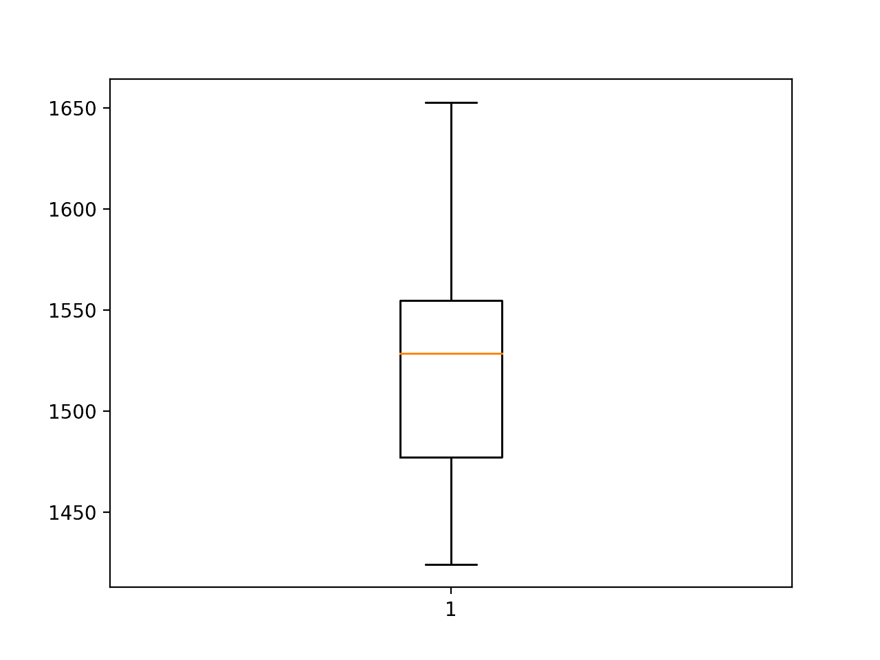 ![Box and Whisker Plot of Convolutional Neural Network RMSE Forecasting Car Sales](https://img.kancloud.cn/92/48/924879581330351e7d4981fdb7f3ea86_1280x960.jpg) 卷積神經網絡 RMSE 預測汽車銷售的盒子和晶須圖 ## 循環神經網絡模型循環神經網絡或 RNN 是那些類型的神經網絡，其使用來自先前步驟的網絡輸出作為輸入以嘗試跨序列數據自動學習。長短期內存或 LSTM 網絡是一種 RNN，其實現解決了在序列數據上訓練 RNN 導致穩定模型的一般困難。它通過學習控制每個節點內的循環連接的內部門的權重來實現這一點。盡管針對序列數據進行了開發， [LSTM 尚未證明在時間序列預測問題上有效](https://machinelearningmastery.com/suitability-long-short-term-memory-networks-time-series-forecasting/)，其中輸出是近期觀測的函數，例如自動回歸類型預測問題，例如汽車銷售數據集。然而，我們可以開發用于自回歸問題的 LSTM 模型，并將其用作與其他神經網絡模型進行比較的點。在本節中，我們將探討 LSTM 模型的三變量，用于單變量時間序列預測;他們是： * **LSTM** ：LSTM 網絡原樣。 * **CNN-LSTM** ：學習輸入功能的 CNN 網絡和解釋它們的 LSTM。 * **ConvLSTM** ：CNN 和 LSTM 的組合，其中 LSTM 單元使用 CNN 的卷積過程讀取輸入數據。 ### LSTM LSTM 神經網絡可用于單變量時間序列預測。作為 RNN，它將一次一步地讀取輸入序列的每個時間步長。 LSTM 具有內部存儲器，允許它在讀取給定輸入序列的步驟時累積內部狀態。在序列結束時，隱藏 LSTM 單元層中的每個節點將輸出單個值。該值向量總結了 LSTM 從輸入序列中學習或提取的內容。這可以在完成最終預測之前由完全連接的層解釋。 ```py # define model model = Sequential() model.add(LSTM(n_nodes, activation='relu', input_shape=(n_input, 1))) model.add(Dense(n_nodes, activation='relu')) model.add(Dense(1)) model.compile(loss='mse', optimizer='adam') ``` 與 CNN 一樣，LSTM 可以在每個時間步驟支持多個變量或功能。由于汽車銷售數據集在每個時間步都只有一個值，我們可以將其固定為 1，既可以在 input_shape 參數[ _n_input，1_ ]中定義網絡輸入，也可以定義形狀輸入樣本。 ```py train_x = train_x.reshape((train_x.shape[0], train_x.shape[1], 1)) ``` 與不一次一步讀取序列數據的 MLP 和 CNN 不同，如果數據是靜止的，LSTM 確實表現更好。這意味著執行差異操作以消除趨勢和季節性結構。對于汽車銷售數據集，我們可以通過執行季節性調整來制作數據信息，即從每個觀察值中減去一年前的值。 ```py adjusted = value - value[-12] ``` 這可以針對整個訓練數據集系統地執行。這也意味著必須放棄觀察的第一年，因為我們沒有前一年的數據來區分它們。下面的 _ 差異（）_ 函數將使提供的數據集與提供的偏移量不同，稱為差異順序，例如差異順序。 12 前一個月的一年。 ```py # difference dataset def difference(data, interval): return [data[i] - data[i - interval] for i in range(interval, len(data))] ``` 我們可以使差值順序成為模型的超參數，并且只有在提供非零值的情況下才執行操作。下面提供了用于擬合 LSTM 模型的 _model_fit（）_ 函數。該模型需要一個包含五個模型超參數的列表;他們是： * **n_input** ：用作模型輸入的滯后觀察數。 * **n_nodes** ：隱藏層中使用的 LSTM 單元數。 * **n_epochs** ：將模型公開給整個訓練數據集的次數。 * **n_batch** ：更新權重的時期內的樣本數。 * **n_diff** ：差值順序或 0 如果不使用。 ```py # fit a model def model_fit(train, config): # unpack config n_input, n_nodes, n_epochs, n_batch, n_diff = config # prepare data if n_diff > 0: train = difference(train, n_diff) data = series_to_supervised(train, n_in=n_input) train_x, train_y = data[:, :-1], data[:, -1] train_x = train_x.reshape((train_x.shape[0], train_x.shape[1], 1)) # define model model = Sequential() model.add(LSTM(n_nodes, activation='relu', input_shape=(n_input, 1))) model.add(Dense(n_nodes, activation='relu')) model.add(Dense(1)) model.compile(loss='mse', optimizer='adam') # fit model.fit(train_x, train_y, epochs=n_epochs, batch_size=n_batch, verbose=0) return model ``` 使用 LSTM 模型進行預測與使用 CNN 模型進行預測相同。單個輸入必須具有樣本，時間步長和特征的三維結構，在這種情況下，我們只有 1 個樣本和 1 個特征：[ _1，n_input，1_ ]。如果執行差異操作，我們必須添加模型進行預測后減去的值。在制定用于進行預測的單個輸入之前，我們還必須區分歷史數據。下面的 _model_predict（）_ 函數實現了這種行為。 ```py # forecast with a pre-fit model def model_predict(model, history, config): # unpack config n_input, _, _, _, n_diff = config # prepare data correction = 0.0 if n_diff > 0: correction = history[-n_diff] history = difference(history, n_diff) x_input = array(history[-n_input:]).reshape((1, n_input, 1)) # forecast yhat = model.predict(x_input, verbose=0) return correction + yhat[0] ``` 進行模型超參數的簡單網格搜索，并選擇下面的配置。這不是最佳配置，但卻是最好的配置。所選配置如下： * **n_input** ：36（即 3 年或 3 * 12） * **n_nodes** ：50 * **n_epochs** ：100 * **n_batch** ：100（即批量梯度下降） * **n_diff** ：12（即季節性差異）這可以指定為一個列表： ```py # define config config = [36, 50, 100, 100, 12] ``` 將所有這些結合在一起，下面列出了完整的示例。 ```py # evaluate lstm from math import sqrt from numpy import array from numpy import mean from numpy import std from pandas import DataFrame from pandas import concat from pandas import read_csv from sklearn.metrics import mean_squared_error from keras.models import Sequential from keras.layers import Dense from keras.layers import LSTM from matplotlib import pyplot # split a univariate dataset into train/test sets def train_test_split(data, n_test): return data[:-n_test], data[-n_test:] # transform list into supervised learning format def series_to_supervised(data, n_in=1, n_out=1): df = DataFrame(data) cols = list() # input sequence (t-n, ... t-1) for i in range(n_in, 0, -1): cols.append(df.shift(i)) # forecast sequence (t, t+1, ... t+n) for i in range(0, n_out): cols.append(df.shift(-i)) # put it all together agg = concat(cols, axis=1) # drop rows with NaN values agg.dropna(inplace=True) return agg.values # root mean squared error or rmse def measure_rmse(actual, predicted): return sqrt(mean_squared_error(actual, predicted)) # difference dataset def difference(data, interval): return [data[i] - data[i - interval] for i in range(interval, len(data))] # fit a model def model_fit(train, config): # unpack config n_input, n_nodes, n_epochs, n_batch, n_diff = config # prepare data if n_diff > 0: train = difference(train, n_diff) data = series_to_supervised(train, n_in=n_input) train_x, train_y = data[:, :-1], data[:, -1] train_x = train_x.reshape((train_x.shape[0], train_x.shape[1], 1)) # define model model = Sequential() model.add(LSTM(n_nodes, activation='relu', input_shape=(n_input, 1))) model.add(Dense(n_nodes, activation='relu')) model.add(Dense(1)) model.compile(loss='mse', optimizer='adam') # fit model.fit(train_x, train_y, epochs=n_epochs, batch_size=n_batch, verbose=0) return model # forecast with a pre-fit model def model_predict(model, history, config): # unpack config n_input, _, _, _, n_diff = config # prepare data correction = 0.0 if n_diff > 0: correction = history[-n_diff] history = difference(history, n_diff) x_input = array(history[-n_input:]).reshape((1, n_input, 1)) # forecast yhat = model.predict(x_input, verbose=0) return correction + yhat[0] # walk-forward validation for univariate data def walk_forward_validation(data, n_test, cfg): predictions = list() # split dataset train, test = train_test_split(data, n_test) # fit model model = model_fit(train, cfg) # seed history with training dataset history = [x for x in train] # step over each time-step in the test set for i in range(len(test)): # fit model and make forecast for history yhat = model_predict(model, history, cfg) # store forecast in list of predictions predictions.append(yhat) # add actual observation to history for the next loop history.append(test[i]) # estimate prediction error error = measure_rmse(test, predictions) print(' > %.3f' % error) return error # repeat evaluation of a config def repeat_evaluate(data, config, n_test, n_repeats=30): # fit and evaluate the model n times scores = [walk_forward_validation(data, n_test, config) for _ in range(n_repeats)] return scores # summarize model performance def summarize_scores(name, scores): # print a summary scores_m, score_std = mean(scores), std(scores) print('%s: %.3f RMSE (+/- %.3f)' % (name, scores_m, score_std)) # box and whisker plot pyplot.boxplot(scores) pyplot.show() series = read_csv('monthly-car-sales.csv', header=0, index_col=0) data = series.values # data split n_test = 12 # define config config = [36, 50, 100, 100, 12] # grid search scores = repeat_evaluate(data, config, n_test) # summarize scores summarize_scores('lstm', scores) ``` 運行該示例，我們可以看到每次重復評估模型的 RMSE。在運行結束時，我們可以看到平均 RMSE 約為 2,109，這比樸素模型更差。這表明所選擇的模型并不熟練，并且鑒于前面部分中用于查找模型配置的相同資源，它是最好的。這提供了進一步的證據（雖然證據不足），LSTM，至少單獨，可能不適合自回歸型序列預測問題。 ```py > 2129.480 > 2169.109 > 2078.290 > 2257.222 > 2014.911 > 2197.283 > 2028.176 > 2110.718 > 2100.388 > 2157.271 > 1940.103 > 2086.588 > 1986.696 > 2168.784 > 2188.813 > 2086.759 > 2128.095 > 2126.467 > 2077.463 > 2057.679 > 2209.818 > 2067.082 > 1983.346 > 2157.749 > 2145.071 > 2266.130 > 2105.043 > 2128.549 > 1952.002 > 2188.287 lstm: 2109.779 RMSE (+/- 81.373) ``` 還創建了一個盒子和胡須圖，總結了 RMSE 分數的分布。甚至模型的基本情況也沒有達到樸素模型的表現。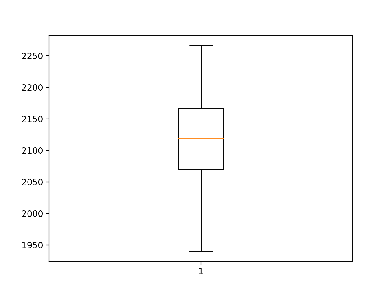 ![Box and Whisker Plot of Long Short-Term Memory Neural Network RMSE Forecasting Car Sales](https://img.kancloud.cn/6e/90/6e90c41d93fc7b98412846786a6534af_1280x960.jpg) 長短期記憶神經網絡 RMSE 預測汽車銷售的盒子和晶須圖 ### CNN LSTM 我們已經看到 CNN 模型能夠自動學習和從原始序列數據中提取特征而無需縮放或差分。我們可以將此功能與 LSTM 結合使用，其中 CNN 模型應用于輸入數據的子序列，其結果一起形成可由 LSTM 模型解釋的提取特征的時間序列。用于通過 LSTM 隨時間讀取多個子序列的 CNN 模型的這種組合稱為 CNN-LSTM 模型。該模型要求每個輸入序列，例如， 36 個月，分為多個子序列，每個子序列由 CNN 模型讀取，例如， 12 個時間步驟的 3 個子序列。將子序列劃分多年可能是有意義的，但這只是一個假設，可以使用其他分裂，例如六個時間步驟的六個子序列。因此，對于子序列的數量和每個子序列參數的步數，使用 _n_seq_ 和 _n_steps_ 參數化該分裂。 ```py train_x = train_x.reshape((train_x.shape[0], n_seq, n_steps, 1)) ``` 每個樣本的滯后觀察數量簡單（ _n_seq * n_steps_ ）。這是一個 4 維輸入數組，現在尺寸為： ```py [samples, subsequences, timesteps, features] ``` 必須對每個輸入子序列應用相同的 CNN 模型。我們可以通過將整個 CNN 模型包裝在 _TimeDistributed_ 層包裝器中來實現這一點。 ```py model = Sequential() model.add(TimeDistributed(Conv1D(filters=n_filters, kernel_size=n_kernel, activation='relu', input_shape=(None,n_steps,1)))) model.add(TimeDistributed(Conv1D(filters=n_filters, kernel_size=n_kernel, activation='relu'))) model.add(TimeDistributed(MaxPooling1D(pool_size=2))) model.add(TimeDistributed(Flatten())) ``` CNN 子模型的一個應用程序的輸出將是向量。子模型到每個輸入子序列的輸出將是可由 LSTM 模型解釋的時間序列的解釋。接下來是完全連接的層，用于解釋 LSTM 的結果，最后是輸出層，用于進行一步預測。 ```py model.add(LSTM(n_nodes, activation='relu')) model.add(Dense(n_nodes, activation='relu')) model.add(Dense(1)) ``` 完整的 _model_fit（）_ 功能如下所示。該模型需要一個包含七個超參數的列表;他們是： * **n_seq** ：樣本中的子序列數。 * **n_steps** ：每個子序列中的時間步數。 * **n_filters** ：并行濾波器的數量。 * **n_kernel** ：每次讀取輸入序列時考慮的時間步數。 * **n_nodes** ：隱藏層中使用的 LSTM 單元數。 * **n_epochs** ：將模型公開給整個訓練數據集的次數。 * **n_batch** ：更新權重的時期內的樣本數。 ```py # fit a model def model_fit(train, config): # unpack config n_seq, n_steps, n_filters, n_kernel, n_nodes, n_epochs, n_batch = config n_input = n_seq * n_steps # prepare data data = series_to_supervised(train, n_in=n_input) train_x, train_y = data[:, :-1], data[:, -1] train_x = train_x.reshape((train_x.shape[0], n_seq, n_steps, 1)) # define model model = Sequential() model.add(TimeDistributed(Conv1D(filters=n_filters, kernel_size=n_kernel, activation='relu', input_shape=(None,n_steps,1)))) model.add(TimeDistributed(Conv1D(filters=n_filters, kernel_size=n_kernel, activation='relu'))) model.add(TimeDistributed(MaxPooling1D(pool_size=2))) model.add(TimeDistributed(Flatten())) model.add(LSTM(n_nodes, activation='relu')) model.add(Dense(n_nodes, activation='relu')) model.add(Dense(1)) model.compile(loss='mse', optimizer='adam') # fit model.fit(train_x, train_y, epochs=n_epochs, batch_size=n_batch, verbose=0) return model ``` 使用擬合模型進行預測與 LSTM 或 CNN 大致相同，盡管添加了將每個樣本分成具有給定數量的時間步長的子序列。 ```py # prepare data x_input = array(history[-n_input:]).reshape((1, n_seq, n_steps, 1)) ``` 更新后的 _model_predict（）_ 功能如下所示。 ```py # forecast with a pre-fit model def model_predict(model, history, config): # unpack config n_seq, n_steps, _, _, _, _, _ = config n_input = n_seq * n_steps # prepare data x_input = array(history[-n_input:]).reshape((1, n_seq, n_steps, 1)) # forecast yhat = model.predict(x_input, verbose=0) return yhat[0] ``` 進行模型超參數的簡單網格搜索，并選擇下面的配置。這可能不是最佳配置，但它是最好的配置。 * **n_seq** ：3（即 3 年） * **n_steps** ：12（即 1 個月） * **n_filters** ：64 * **n_kernel** ：3 * **n_nodes** ：100 * **n_epochs** ：200 * **n_batch** ：100（即批量梯度下降）我們可以將配置定義為列表;例如： ```py # define config config = [3, 12, 64, 3, 100, 200, 100] ``` 下面列出了評估用于預測單變量月度汽車銷售的 CNN-LSTM 模型的完整示例。 ```py # evaluate cnn lstm from math import sqrt from numpy import array from numpy import mean from numpy import std from pandas import DataFrame from pandas import concat from pandas import read_csv from sklearn.metrics import mean_squared_error from keras.models import Sequential from keras.layers import Dense from keras.layers import LSTM from keras.layers import TimeDistributed from keras.layers import Flatten from keras.layers.convolutional import Conv1D from keras.layers.convolutional import MaxPooling1D from matplotlib import pyplot # split a univariate dataset into train/test sets def train_test_split(data, n_test): return data[:-n_test], data[-n_test:] # transform list into supervised learning format def series_to_supervised(data, n_in=1, n_out=1): df = DataFrame(data) cols = list() # input sequence (t-n, ... t-1) for i in range(n_in, 0, -1): cols.append(df.shift(i)) # forecast sequence (t, t+1, ... t+n) for i in range(0, n_out): cols.append(df.shift(-i)) # put it all together agg = concat(cols, axis=1) # drop rows with NaN values agg.dropna(inplace=True) return agg.values # root mean squared error or rmse def measure_rmse(actual, predicted): return sqrt(mean_squared_error(actual, predicted)) # fit a model def model_fit(train, config): # unpack config n_seq, n_steps, n_filters, n_kernel, n_nodes, n_epochs, n_batch = config n_input = n_seq * n_steps # prepare data data = series_to_supervised(train, n_in=n_input) train_x, train_y = data[:, :-1], data[:, -1] train_x = train_x.reshape((train_x.shape[0], n_seq, n_steps, 1)) # define model model = Sequential() model.add(TimeDistributed(Conv1D(filters=n_filters, kernel_size=n_kernel, activation='relu', input_shape=(None,n_steps,1)))) model.add(TimeDistributed(Conv1D(filters=n_filters, kernel_size=n_kernel, activation='relu'))) model.add(TimeDistributed(MaxPooling1D(pool_size=2))) model.add(TimeDistributed(Flatten())) model.add(LSTM(n_nodes, activation='relu')) model.add(Dense(n_nodes, activation='relu')) model.add(Dense(1)) model.compile(loss='mse', optimizer='adam') # fit model.fit(train_x, train_y, epochs=n_epochs, batch_size=n_batch, verbose=0) return model # forecast with a pre-fit model def model_predict(model, history, config): # unpack config n_seq, n_steps, _, _, _, _, _ = config n_input = n_seq * n_steps # prepare data x_input = array(history[-n_input:]).reshape((1, n_seq, n_steps, 1)) # forecast yhat = model.predict(x_input, verbose=0) return yhat[0] # walk-forward validation for univariate data def walk_forward_validation(data, n_test, cfg): predictions = list() # split dataset train, test = train_test_split(data, n_test) # fit model model = model_fit(train, cfg) # seed history with training dataset history = [x for x in train] # step over each time-step in the test set for i in range(len(test)): # fit model and make forecast for history yhat = model_predict(model, history, cfg) # store forecast in list of predictions predictions.append(yhat) # add actual observation to history for the next loop history.append(test[i]) # estimate prediction error error = measure_rmse(test, predictions) print(' > %.3f' % error) return error # repeat evaluation of a config def repeat_evaluate(data, config, n_test, n_repeats=30): # fit and evaluate the model n times scores = [walk_forward_validation(data, n_test, config) for _ in range(n_repeats)] return scores # summarize model performance def summarize_scores(name, scores): # print a summary scores_m, score_std = mean(scores), std(scores) print('%s: %.3f RMSE (+/- %.3f)' % (name, scores_m, score_std)) # box and whisker plot pyplot.boxplot(scores) pyplot.show() series = read_csv('monthly-car-sales.csv', header=0, index_col=0) data = series.values # data split n_test = 12 # define config config = [3, 12, 64, 3, 100, 200, 100] # grid search scores = repeat_evaluate(data, config, n_test) # summarize scores summarize_scores('cnn-lstm', scores) ``` 運行該示例為每次重復的模型評估打印 RMSE。最終平均 RMSE 報告在約 1,626 的末尾，低于幼稚模型，但仍高于 SARIMA 模型。該分數的標準偏差也非常大，表明所選配置可能不如獨立 CNN 模型穩定。 ```py > 1543.533 > 1421.895 > 1467.927 > 1441.125 > 1750.995 > 1321.498 > 1571.657 > 1845.298 > 1621.589 > 1425.065 > 1675.232 > 1807.288 > 2922.295 > 1391.861 > 1626.655 > 1633.177 > 1667.572 > 1577.285 > 1590.235 > 1557.385 > 1784.982 > 1664.839 > 1741.729 > 1437.992 > 1772.076 > 1289.794 > 1685.976 > 1498.123 > 1618.627 > 1448.361 cnn-lstm: 1626.735 RMSE (+/- 279.850) ``` 還創建了一個盒子和胡須圖，總結了 RMSE 分數的分布。該圖顯示了一個非常差的表現異常值，僅低于 3,000 個銷售額。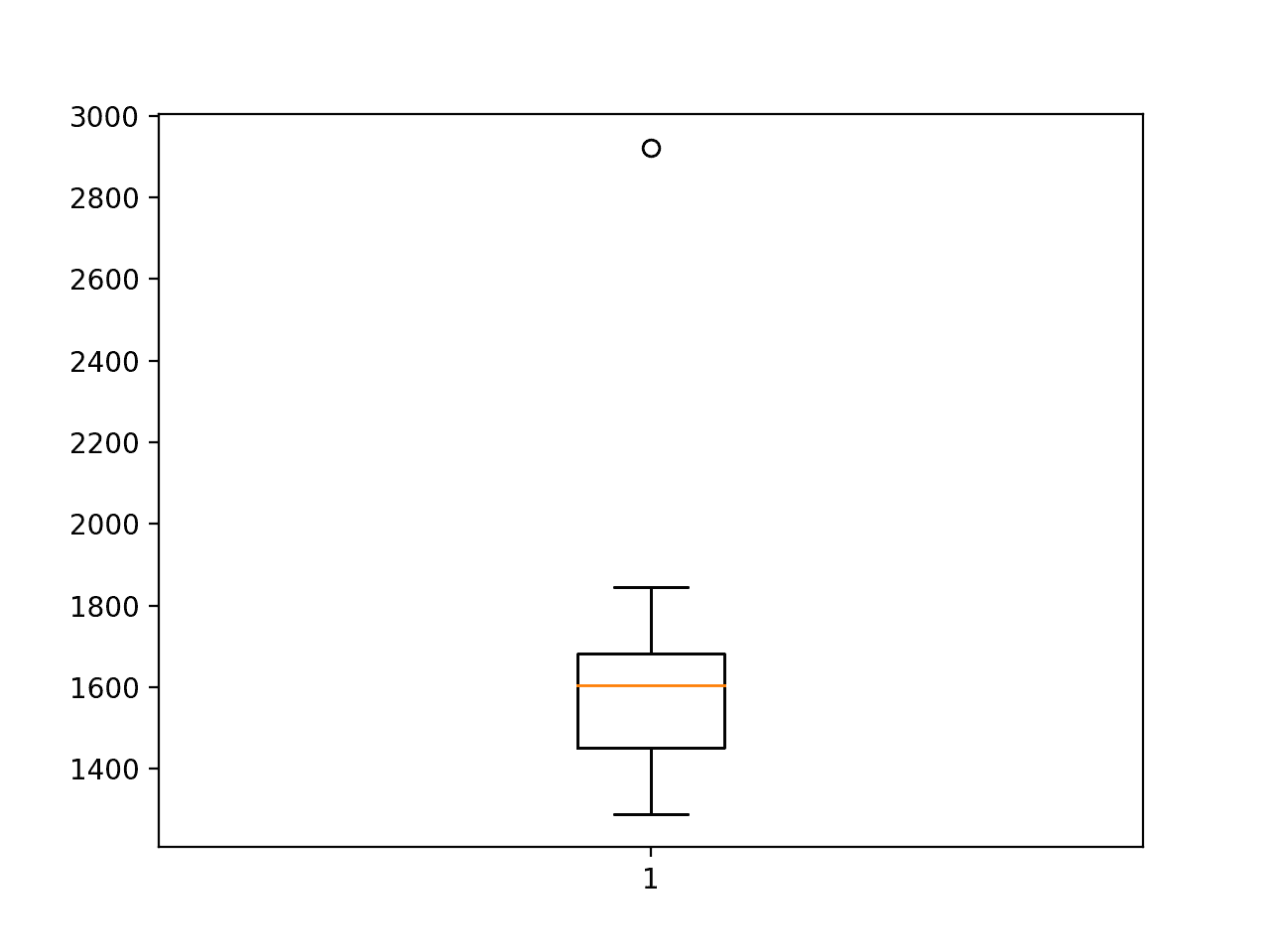 ![Box and Whisker Plot of CNN-LSTM RMSE Forecasting Car Sales](https://img.kancloud.cn/ac/73/ac73235e54d1672b20f36b43031ed759_1280x960.jpg) CNN-LSTM RMSE 預測汽車銷售的盒子和晶須圖 ### ConvLSTM 作為讀取每個 LSTM 單元內的輸入序列的一部分，可以執行卷積運算。這意味著，LSTM 不是一次一步地讀取序列，而是使用卷積過程（如 CNN）一次讀取觀察的塊或子序列。這與使用 LSTM 首先讀取提取特征并使用 LSTM 解釋結果不同;這是作為 LSTM 的一部分在每個時間步執行 CNN 操作。這種類型的模型稱為卷積 LSTM，簡稱 ConvLSTM。它在 Keras 中作為 2D 數據稱為 ConvLSTM2D 的層提供。我們可以通過假設我們有一行包含多列來配置它以用于 1D 序列數據。與 CNN-LSTM 一樣，輸入數據被分成子序列，其中每個子序列具有固定數量的時間步長，盡管我們還必須指定每個子序列中的行數，在這種情況下固定為 1。 ```py train_x = train_x.reshape((train_x.shape[0], n_seq, 1, n_steps, 1)) ``` 形狀是五維的，尺寸為： ```py [samples, subsequences, rows, columns, features] ``` 與 CNN 一樣，ConvLSTM 層允許我們指定過濾器映射的數量以及讀取輸入序列時使用的內核的大小。 ```py model.add(ConvLSTM2D(filters=n_filters, kernel_size=(1,n_kernel), activation='relu', input_shape=(n_seq, 1, n_steps, 1))) ``` 層的輸出是一系列過濾器映射，在解釋之前必須首先將其展平，然后是輸出層。該模型需要一個包含七個超參數的列表，與 CNN-LSTM 相同;他們是： * **n_seq** ：樣本中的子序列數。 * **n_steps** ：每個子序列中的時間步數。 * **n_filters** ：并行濾波器的數量。 * **n_kernel** ：每次讀取輸入序列時考慮的時間步數。 * **n_nodes** ：隱藏層中使用的 LSTM 單元數。 * **n_epochs** ：將模型公開給整個訓練數據集的次數。 * **n_batch** ：更新權重的時期內的樣本數。下面列出了實現所有這些功能的 _model_fit（）_ 函數。 ```py # fit a model def model_fit(train, config): # unpack config n_seq, n_steps, n_filters, n_kernel, n_nodes, n_epochs, n_batch = config n_input = n_seq * n_steps # prepare data data = series_to_supervised(train, n_in=n_input) train_x, train_y = data[:, :-1], data[:, -1] train_x = train_x.reshape((train_x.shape[0], n_seq, 1, n_steps, 1)) # define model model = Sequential() model.add(ConvLSTM2D(filters=n_filters, kernel_size=(1,n_kernel), activation='relu', input_shape=(n_seq, 1, n_steps, 1))) model.add(Flatten()) model.add(Dense(n_nodes, activation='relu')) model.add(Dense(1)) model.compile(loss='mse', optimizer='adam') # fit model.fit(train_x, train_y, epochs=n_epochs, batch_size=n_batch, verbose=0) return model ``` 使用擬合模型以與 CNN-LSTM 相同的方式進行預測，盡管我們將附加行維度固定為 1。 ```py # prepare data x_input = array(history[-n_input:]).reshape((1, n_seq, 1, n_steps, 1)) ``` 下面列出了用于進行單個一步預測的 _model_predict（）_ 函數。 ```py # forecast with a pre-fit model def model_predict(model, history, config): # unpack config n_seq, n_steps, _, _, _, _, _ = config n_input = n_seq * n_steps # prepare data x_input = array(history[-n_input:]).reshape((1, n_seq, 1, n_steps, 1)) # forecast yhat = model.predict(x_input, verbose=0) return yhat[0] ``` 進行模型超參數的簡單網格搜索，并選擇下面的配置。這可能不是最佳配置，但卻是最好的配置。 * **n_seq** ：3（即 3 年） * **n_steps** ：12（即 1 個月） * **n_filters** ：256 * **n_kernel** ：3 * **n_nodes** ：200 * **n_epochs** ：200 * **n_batch** ：100（即批量梯度下降）我們可以將配置定義為列表;例如： ```py # define config config = [3, 12, 256, 3, 200, 200, 100] ``` 我們可以將所有這些結合在一起。下面列出了評估每月汽車銷售數據集一步預測的 ConvLSTM 模型的完整代碼清單。 ```py # evaluate convlstm from math import sqrt from numpy import array from numpy import mean from numpy import std from pandas import DataFrame from pandas import concat from pandas import read_csv from sklearn.metrics import mean_squared_error from keras.models import Sequential from keras.layers import Dense from keras.layers import Flatten from keras.layers import ConvLSTM2D from matplotlib import pyplot # split a univariate dataset into train/test sets def train_test_split(data, n_test): return data[:-n_test], data[-n_test:] # transform list into supervised learning format def series_to_supervised(data, n_in=1, n_out=1): df = DataFrame(data) cols = list() # input sequence (t-n, ... t-1) for i in range(n_in, 0, -1): cols.append(df.shift(i)) # forecast sequence (t, t+1, ... t+n) for i in range(0, n_out): cols.append(df.shift(-i)) # put it all together agg = concat(cols, axis=1) # drop rows with NaN values agg.dropna(inplace=True) return agg.values # root mean squared error or rmse def measure_rmse(actual, predicted): return sqrt(mean_squared_error(actual, predicted)) # difference dataset def difference(data, interval): return [data[i] - data[i - interval] for i in range(interval, len(data))] # fit a model def model_fit(train, config): # unpack config n_seq, n_steps, n_filters, n_kernel, n_nodes, n_epochs, n_batch = config n_input = n_seq * n_steps # prepare data data = series_to_supervised(train, n_in=n_input) train_x, train_y = data[:, :-1], data[:, -1] train_x = train_x.reshape((train_x.shape[0], n_seq, 1, n_steps, 1)) # define model model = Sequential() model.add(ConvLSTM2D(filters=n_filters, kernel_size=(1,n_kernel), activation='relu', input_shape=(n_seq, 1, n_steps, 1))) model.add(Flatten()) model.add(Dense(n_nodes, activation='relu')) model.add(Dense(1)) model.compile(loss='mse', optimizer='adam') # fit model.fit(train_x, train_y, epochs=n_epochs, batch_size=n_batch, verbose=0) return model # forecast with a pre-fit model def model_predict(model, history, config): # unpack config n_seq, n_steps, _, _, _, _, _ = config n_input = n_seq * n_steps # prepare data x_input = array(history[-n_input:]).reshape((1, n_seq, 1, n_steps, 1)) # forecast yhat = model.predict(x_input, verbose=0) return yhat[0] # walk-forward validation for univariate data def walk_forward_validation(data, n_test, cfg): predictions = list() # split dataset train, test = train_test_split(data, n_test) # fit model model = model_fit(train, cfg) # seed history with training dataset history = [x for x in train] # step over each time-step in the test set for i in range(len(test)): # fit model and make forecast for history yhat = model_predict(model, history, cfg) # store forecast in list of predictions predictions.append(yhat) # add actual observation to history for the next loop history.append(test[i]) # estimate prediction error error = measure_rmse(test, predictions) print(' > %.3f' % error) return error # repeat evaluation of a config def repeat_evaluate(data, config, n_test, n_repeats=30): # fit and evaluate the model n times scores = [walk_forward_validation(data, n_test, config) for _ in range(n_repeats)] return scores # summarize model performance def summarize_scores(name, scores): # print a summary scores_m, score_std = mean(scores), std(scores) print('%s: %.3f RMSE (+/- %.3f)' % (name, scores_m, score_std)) # box and whisker plot pyplot.boxplot(scores) pyplot.show() series = read_csv('monthly-car-sales.csv', header=0, index_col=0) data = series.values # data split n_test = 12 # define config config = [3, 12, 256, 3, 200, 200, 100] # grid search scores = repeat_evaluate(data, config, n_test) # summarize scores summarize_scores('convlstm', scores) ``` 運行該示例為每次重復的模型評估打印 RMSE。最終的平均 RMSE 報告在約 1,660 結束時，低于幼稚模型，但仍高于 SARIMA 模型。這個結果可能與 CNN-LSTM 模型相當。該分數的標準偏差也非常大，表明所選配置可能不如獨立 CNN 模型穩定。 ```py > 1825.246 > 1862.674 > 1684.313 > 1310.448 > 2109.668 > 1507.912 > 1431.118 > 1442.692 > 1400.548 > 1732.381 > 1523.824 > 1611.898 > 1805.970 > 1616.015 > 1649.466 > 1521.884 > 2025.655 > 1622.886 > 2536.448 > 1526.532 > 1866.631 > 1562.625 > 1491.386 > 1506.270 > 1843.981 > 1653.084 > 1650.430 > 1291.353 > 1558.616 > 1653.231 convlstm: 1660.840 RMSE (+/- 248.826) ``` 還創建了一個盒子和胡須圖，總結了 RMSE 分數的分布。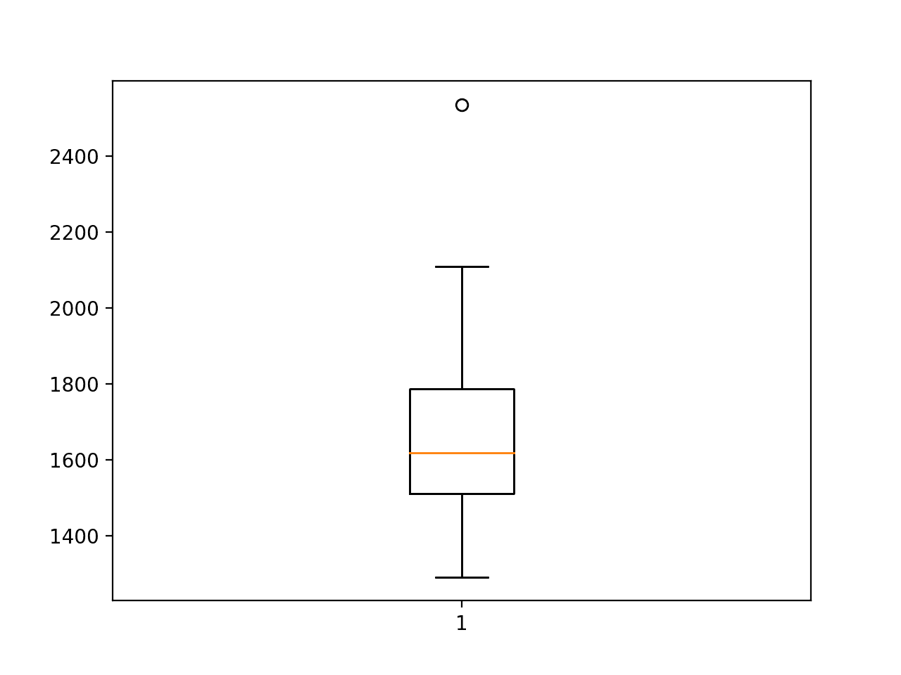 ![Box and Whisker Plot of ConvLSTM RMSE Forecasting Car Sales](https://img.kancloud.cn/3c/83/3c833ac433c04b874be233bd8c47ffab_1280x960.jpg) ConvLSTM RMSE 預測汽車銷售的盒子和晶須圖 ## 擴展本節列出了一些擴展您可能希望探索的教程的想法。 * **數據準備**。探索數據準備（例如規范化，標準化和/或差異化）是否可以列出任何模型的表現。 * **網格搜索超參數**。對一個模型實施超參數的網格搜索，以查看是否可以進一步提升表現。 * **學習曲線診斷**。創建一個模型的單一擬合并查看數據集的訓練和驗證分割的學習曲線，然后使用學習曲線的診斷來進一步調整模型超參數以提高模型表現。 * **歷史規模**。探索一種模型的不同數量的歷史數據（滯后輸入），以了解您是否可以進一步提高模型表現 * **減少最終模型的差異**。探索一種或多種策略來減少其中一種神經網絡模型的方差。 * **前進期間更新**。探索作為前進驗證的一部分重新擬合或更新神經網絡模型是否可以進一步提高模型表現。 * **更多參數化**。探索為一個模型添加更多模型參數化，例如使用其他層。如果你探索任何這些擴展，我很想知道。 ## 進一步閱讀如果您希望深入了解，本節將提供有關該主題的更多資源。 * [pandas.DataFrame.shift API](http://pandas-docs.github.io/pandas-docs-travis/generated/pandas.DataFrame.shift.html) * [sklearn.metrics.mean_squared_error API](http://scikit-learn.org/stable/modules/generated/sklearn.metrics.mean_squared_error.html) * [matplotlib.pyplot.boxplot API](https://matplotlib.org/api/_as_gen/matplotlib.pyplot.boxplot.html) * [Keras 序列模型 API](https://keras.io/models/sequential/) ## 摘要在本教程中，您了解了如何開發一套用于單變量時間序列預測的深度學習模型。具體來說，你學到了： * 如何使用前向驗證開發一個強大的測試工具來評估神經網絡模型的表現。 * 如何開發和評估簡單多層感知器和卷積神經網絡的時間序列預測。 * 如何開發和評估 LSTM，CNN-LSTM 和 ConvLSTM 神經網絡模型用于時間序列預測。你有任何問題嗎？在下面的評論中提出您的問題，我會盡力回答。