# 如何利用 LSTM 網絡進行權重正則化進行時間序列預測 > 原文： [https://machinelearningmastery.com/use-weight-regularization-lstm-networks-time-series-forecasting/](https://machinelearningmastery.com/use-weight-regularization-lstm-networks-time-series-forecasting/) 長短期記憶（LSTM）模型是能夠學習觀察序列的循環神經網絡。 這可能使它們成為一個非常適合時間序列預測的網絡。 LSTM 的一個問題是他們可以輕松地過度訓練訓練數據，降低他們的預測技巧。 權重正則化是一種對 LSTM 節點內的權重施加約束（例如 L1 或 L2）的技術。這具有減少過度擬合和改善模型表現的效果。 在本教程中，您將了解如何使用 LSTM 網絡進行權重正則化，并設計實驗來測試其對時間序列預測的有效性。 完成本教程后，您將了解： * 如何設計一個強大的測試工具來評估 LSTM 網絡的時間序列預測。 * 如何設計，執行和解釋使用 LSTM 的偏置權重正則化的結果。 * 如何設計，執行和解釋使用 LSTM 的輸入和循環權重正則化的結果。 讓我們開始吧。  如何使用 LSTM 網絡進行權重正則化進行時間序列預測 攝影：Julian Fong，保留一些權利。 ## 教程概述 本教程分為 6 個部分。他們是： 1. 洗發水銷售數據集 2. 實驗測試線束 3. 偏差權重正則化 4. 輸入權重正則化 5. 復發性體重正則化 6. 審查結果 ### 環境 本教程假定您已安裝 Python SciPy 環境。您可以在此示例中使用 Python 2 或 3。 本教程假設您安裝了 TensorFlow 或 Theano 后端的 Keras v2.0 或更高版本。 本教程還假設您安裝了 scikit-learn，Pandas，NumPy 和 Matplotlib。 如果您在設置 Python 環境時需要幫助，請參閱以下帖子： * [如何使用 Anaconda 設置用于機器學習和深度學習的 Python 環境](http://machinelearningmastery.com/setup-python-environment-machine-learning-deep-learning-anaconda/) 接下來，讓我們看看標準時間序列預測問題，我們可以將其用作此實驗的上下文。 ## 洗發水銷售數據集 該數據集描述了 3 年期間每月洗發水的銷售數量。 單位是銷售計數，有 36 個觀察。原始數據集歸功于 Makridakis，Wheelwright 和 Hyndman（1998）。 [您可以在此處下載并了解有關數據集的更多信息](https://datamarket.com/data/set/22r0/sales-of-shampoo-over-a-three-year-period)。 下面的示例加載并創建已加載數據集的圖。 ```py # load and plot dataset from pandas import read_csv from pandas import datetime from matplotlib import pyplot # load dataset def parser(x): return datetime.strptime('190'+x, '%Y-%m') series = read_csv('shampoo-sales.csv', header=0, parse_dates=[0], index_col=0, squeeze=True, date_parser=parser) # summarize first few rows print(series.head()) # line plot series.plot() pyplot.show() ``` 運行該示例將數據集作為 Pandas Series 加載并打印前 5 行。 ```py Month 1901-01-01 266.0 1901-02-01 145.9 1901-03-01 183.1 1901-04-01 119.3 1901-05-01 180.3 Name: Sales, dtype: float64 ``` 然后創建該系列的線圖，顯示明顯的增加趨勢。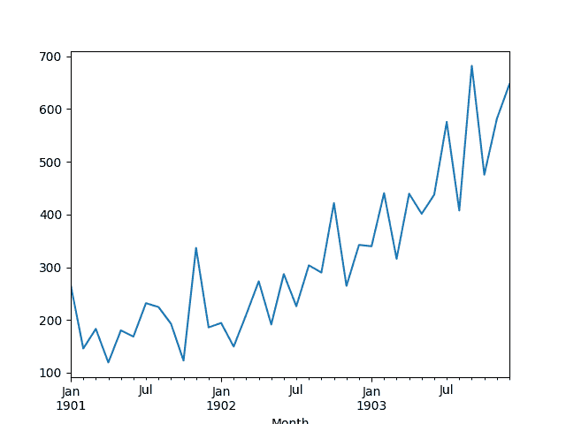  洗發水銷售數據集的線圖 接下來，我們將看一下實驗中使用的模型配置和測試工具。 ## 實驗測試線束 本節介紹本教程中使用的測試工具。 ### 數據拆分 我們將 Shampoo Sales 數據集分為兩部分：訓練和測試集。 前兩年的數據將用于訓練數據集，剩余的一年數據將用于測試集。 將使用訓練數據集開發模型，并對測試數據集進行預測。 測試數據集的持久性預測（樸素預測）實現了每月洗發水銷售 136.761 的錯誤。這在測試集上提供了較低的可接受表現限制。 ### 模型評估 將使用滾動預測場景，也稱為前進模型驗證。 測試數據集的每個時間步驟將一次一個地走。將使用模型對時間步長進行預測，然后將獲取測試集的實際預期值，并使其可用于下一時間步的預測模型。 這模仿了一個真實世界的場景，每個月都會有新的洗發水銷售觀察結果，并用于下個月的預測。 這將通過訓練和測試數據集的結構進行模擬。 將收集關于測試數據集的所有預測，并計算錯誤分數以總結模型的技能。將使用均方根誤差（RMSE），因為它會對大錯誤進行處罰，并產生與預測數據相同的分數，即每月洗發水銷售額。 ### 數據準備 在我們將模型擬合到數據集之前，我們必須轉換數據。 在擬合模型和進行預測之前，對數據集執行以下三個數據變換。 1. 轉換時間序列數據，使其靜止不動。具體而言，滯后= 1 差分以消除數據中的增加趨勢。 2. 將時間序列轉換為監督學習問題。具體而言，將數據組織成輸入和輸出模式，其中前一時間步的觀察被用作預測當前時間步的觀察的輸入 3. 將觀察結果轉換為具有特定比例。具體而言，將數據重新調整為-1 到 1 之間的值。 這些變換在預測時反轉，在計算和誤差分數之前將它們恢復到原始比例。 ### LSTM 模型 我們將使用基礎狀態 LSTM 模型，其中 1 個神經元適合 1000 個時期。 理想情況下，批量大小為 1 將用于步行前導驗證。我們將假設前進驗證并預測全年的速度。因此，我們可以使用任何可以按樣本數量分割的批量大小，在這種情況下，我們將使用值 4。 理想情況下，將使用更多的訓練時期（例如 1500），但這被截斷為 1000 以保持運行時間合理。 使用有效的 ADAM 優化算法和均方誤差損失函數來擬合模型。 ### 實驗運行 每個實驗場景將運行 30 次，并且測試集上的 RMSE 得分將從每次運行結束時記錄。 讓我們深入研究實驗。 ## 基線 LSTM 模型 讓我們從基線 LSTM 模型開始。 此問題的基線 LSTM 模型具有以下配置： * 滯后輸入：1 * 時代：1000 * LSTM 隱藏層中的單位：3 * 批量大小：4 * 重復：3 完整的代碼清單如下。 此代碼清單將用作所有后續實驗的基礎，后續部分中僅提供對此代碼的更改。 ```py from pandas import DataFrame from pandas import Series from pandas import concat from pandas import read_csv from pandas import datetime from sklearn.metrics import mean_squared_error from sklearn.preprocessing import MinMaxScaler from keras.models import Sequential from keras.layers import Dense from keras.layers import LSTM from keras.regularizers import L1L2 from math import sqrt import matplotlib # be able to save images on server matplotlib.use('Agg') from matplotlib import pyplot import numpy # date-time parsing function for loading the dataset def parser(x): return datetime.strptime('190'+x, '%Y-%m') # frame a sequence as a supervised learning problem def timeseries_to_supervised(data, lag=1): df = DataFrame(data) columns = [df.shift(i) for i in range(1, lag+1)] columns.append(df) df = concat(columns, axis=1) return df # create a differenced series def difference(dataset, interval=1): diff = list() for i in range(interval, len(dataset)): value = dataset[i] - dataset[i - interval] diff.append(value) return Series(diff) # invert differenced value def inverse_difference(history, yhat, interval=1): return yhat + history[-interval] # scale train and test data to [-1, 1] def scale(train, test): # fit scaler scaler = MinMaxScaler(feature_range=(-1, 1)) scaler = scaler.fit(train) # transform train train = train.reshape(train.shape[0], train.shape[1]) train_scaled = scaler.transform(train) # transform test test = test.reshape(test.shape[0], test.shape[1]) test_scaled = scaler.transform(test) return scaler, train_scaled, test_scaled # inverse scaling for a forecasted value def invert_scale(scaler, X, yhat): new_row = [x for x in X] + [yhat] array = numpy.array(new_row) array = array.reshape(1, len(array)) inverted = scaler.inverse_transform(array) return inverted[0, -1] # fit an LSTM network to training data def fit_lstm(train, n_batch, nb_epoch, n_neurons): X, y = train[:, 0:-1], train[:, -1] X = X.reshape(X.shape[0], 1, X.shape[1]) model = Sequential() model.add(LSTM(n_neurons, batch_input_shape=(n_batch, X.shape[1], X.shape[2]), stateful=True)) model.add(Dense(1)) model.compile(loss='mean_squared_error', optimizer='adam') for i in range(nb_epoch): model.fit(X, y, epochs=1, batch_size=n_batch, verbose=0, shuffle=False) model.reset_states() return model # run a repeated experiment def experiment(series, n_lag, n_repeats, n_epochs, n_batch, n_neurons): # transform data to be stationary raw_values = series.values diff_values = difference(raw_values, 1) # transform data to be supervised learning supervised = timeseries_to_supervised(diff_values, n_lag) supervised_values = supervised.values[n_lag:,:] # split data into train and test-sets train, test = supervised_values[0:-12], supervised_values[-12:] # transform the scale of the data scaler, train_scaled, test_scaled = scale(train, test) # run experiment error_scores = list() for r in range(n_repeats): # fit the model train_trimmed = train_scaled[2:, :] lstm_model = fit_lstm(train_trimmed, n_batch, n_epochs, n_neurons) # forecast test dataset test_reshaped = test_scaled[:,0:-1] test_reshaped = test_reshaped.reshape(len(test_reshaped), 1, 1) output = lstm_model.predict(test_reshaped, batch_size=n_batch) predictions = list() for i in range(len(output)): yhat = output[i,0] X = test_scaled[i, 0:-1] # invert scaling yhat = invert_scale(scaler, X, yhat) # invert differencing yhat = inverse_difference(raw_values, yhat, len(test_scaled)+1-i) # store forecast predictions.append(yhat) # report performance rmse = sqrt(mean_squared_error(raw_values[-12:], predictions)) print('%d) Test RMSE: %.3f' % (r+1, rmse)) error_scores.append(rmse) return error_scores # configure the experiment def run(): # load dataset series = read_csv('shampoo-sales.csv', header=0, parse_dates=[0], index_col=0, squeeze=True, date_parser=parser) # configure the experiment n_lag = 1 n_repeats = 30 n_epochs = 1000 n_batch = 4 n_neurons = 3 # run the experiment results = DataFrame() results['results'] = experiment(series, n_lag, n_repeats, n_epochs, n_batch, n_neurons) # summarize results print(results.describe()) # save boxplot results.boxplot() pyplot.savefig('experiment_baseline.png') # entry point run() ``` 運行實驗將打印所有重復測試 RMSE 的摘要統計信息。 我們可以看到，平均而言，這種模型配置實現了約 92 個月洗發水銷售的測試 RMSE，標準偏差為 5。 ```py results count 30.000000 mean 92.842537 std 5.748456 min 81.205979 25% 89.514367 50% 92.030003 75% 96.926145 max 105.247117 ``` 還會根據測試 RMSE 結果的分布創建一個盒子和胡須圖并保存到文件中。 該圖清楚地描述了結果的傳播，突出了中間 50％的值（框）和中位數（綠線）。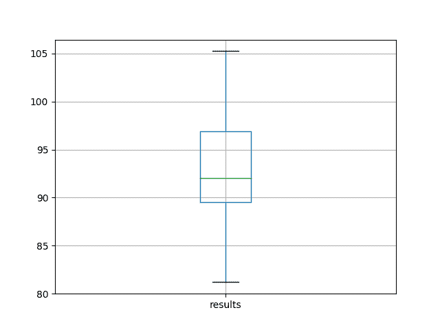  洗發水銷售數據集中基線表現的盒子和晶須圖 ## 偏差權重正則化 權重正則化可以應用于 LSTM 節點內的偏置連接。 在 Keras 中，在創建 LSTM 層時使用 _bias_regularizer_ 參數指定。正則化器被定義為 L1，L2 或 L1L2 類之一的實例。 更多細節在這里： * [Keras 用于規范制定者](https://keras.io/regularizers/) 在本實驗中，我們將 L1，L2 和 L1L2 與基線模型的默認值 0.01 進行比較。我們可以使用 L1L2 類指定所有配置，如下所示： * L1L2（0.0,0.0）[例如基線] * L1L2（0.01,0.0）[例如 L1] * L1L2（0.0,0.01）[例如 L2] * L1L2（0.01,0.01）[例如 L1L2 或彈性網] 下面列出了更新的 _fit_lstm（）_，_ 實驗（）_ 和 _run（）_ 函數，用于使用 LSTM 的偏置權重正則化。 ```py # fit an LSTM network to training data def fit_lstm(train, n_batch, nb_epoch, n_neurons, reg): X, y = train[:, 0:-1], train[:, -1] X = X.reshape(X.shape[0], 1, X.shape[1]) model = Sequential() model.add(LSTM(n_neurons, batch_input_shape=(n_batch, X.shape[1], X.shape[2]), stateful=True, bias_regularizer=reg)) model.add(Dense(1)) model.compile(loss='mean_squared_error', optimizer='adam') for i in range(nb_epoch): model.fit(X, y, epochs=1, batch_size=n_batch, verbose=0, shuffle=False) model.reset_states() return model # run a repeated experiment def experiment(series, n_lag, n_repeats, n_epochs, n_batch, n_neurons, reg): # transform data to be stationary raw_values = series.values diff_values = difference(raw_values, 1) # transform data to be supervised learning supervised = timeseries_to_supervised(diff_values, n_lag) supervised_values = supervised.values[n_lag:,:] # split data into train and test-sets train, test = supervised_values[0:-12], supervised_values[-12:] # transform the scale of the data scaler, train_scaled, test_scaled = scale(train, test) # run experiment error_scores = list() for r in range(n_repeats): # fit the model train_trimmed = train_scaled[2:, :] lstm_model = fit_lstm(train_trimmed, n_batch, n_epochs, n_neurons, reg) # forecast test dataset test_reshaped = test_scaled[:,0:-1] test_reshaped = test_reshaped.reshape(len(test_reshaped), 1, 1) output = lstm_model.predict(test_reshaped, batch_size=n_batch) predictions = list() for i in range(len(output)): yhat = output[i,0] X = test_scaled[i, 0:-1] # invert scaling yhat = invert_scale(scaler, X, yhat) # invert differencing yhat = inverse_difference(raw_values, yhat, len(test_scaled)+1-i) # store forecast predictions.append(yhat) # report performance rmse = sqrt(mean_squared_error(raw_values[-12:], predictions)) print('%d) Test RMSE: %.3f' % (r+1, rmse)) error_scores.append(rmse) return error_scores # configure the experiment def run(): # load dataset series = read_csv('shampoo-sales.csv', header=0, parse_dates=[0], index_col=0, squeeze=True, date_parser=parser) # configure the experiment n_lag = 1 n_repeats = 30 n_epochs = 1000 n_batch = 4 n_neurons = 3 regularizers = [L1L2(l1=0.0, l2=0.0), L1L2(l1=0.01, l2=0.0), L1L2(l1=0.0, l2=0.01), L1L2(l1=0.01, l2=0.01)] # run the experiment results = DataFrame() for reg in regularizers: name = ('l1 %.2f,l2 %.2f' % (reg.l1, reg.l2)) results[name] = experiment(series, n_lag, n_repeats, n_epochs, n_batch, n_neurons, reg) # summarize results print(results.describe()) # save boxplot results.boxplot() pyplot.savefig('experiment_reg_bias.png') ``` 運行此實驗會打印每個已評估配置的描述性統計信息。 結果表明，與所考慮的所有其他配置相比，平均而言，無偏差正則化的默認值導致更好的表現。 ```py l1 0.00,l2 0.00 l1 0.01,l2 0.00 l1 0.00,l2 0.01 l1 0.01,l2 0.01 count 30.000000 30.000000 30.000000 30.000000 mean 92.821489 95.520003 93.285389 92.901021 std 4.894166 3.637022 3.906112 5.082358 min 81.394504 89.477398 82.994480 78.729224 25% 89.356330 93.017723 90.907343 91.210105 50% 92.822871 95.502700 93.837562 94.525965 75% 95.899939 98.195980 95.426270 96.882378 max 101.194678 101.750900 100.650130 97.766301 ``` 還會創建一個框和胡須圖來比較每個配置的結果分布。 該圖顯示所有配置具有大約相同的擴展，并且均勻地添加偏置正則化對該問題沒有幫助。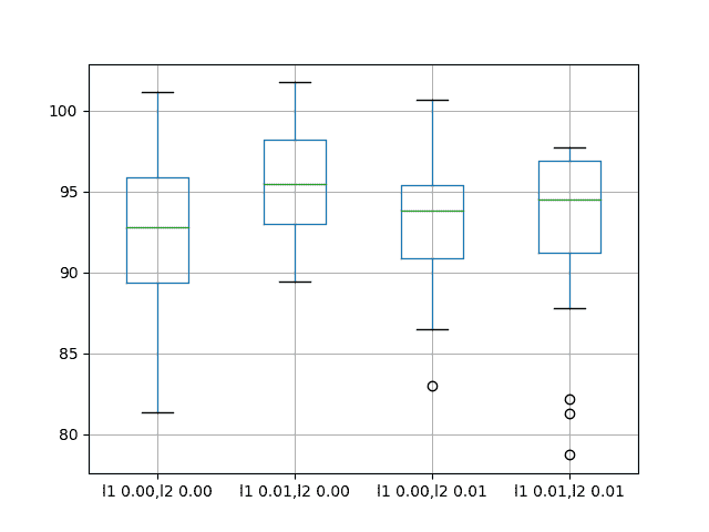  在洗發水銷售數據集中偏差重量正規化的盒子和晶須圖 ## 輸入權重正則化 我們還可以將正則化應用于每個 LSTM 單元上的輸入連接。 在 Keras 中，這是通過將 _kernel_regularizer_ 參數設置為正則化類來實現的。 我們將測試與前一節中使用的相同的正則化器配置，具體為： * L1L2（0.0,0.0）[例如基線] * L1L2（0.01,0.0）[例如 L1] * L1L2（0.0,0.01）[例如 L2] * L1L2（0.01,0.01）[例如 L1L2 或彈性網] 下面列出了更新的 _fit_lstm（）_，_ 實驗（）_ 和 _run（）_ 函數，用于使用 LSTM 的偏置權重正則化。 ```py # fit an LSTM network to training data def fit_lstm(train, n_batch, nb_epoch, n_neurons, reg): X, y = train[:, 0:-1], train[:, -1] X = X.reshape(X.shape[0], 1, X.shape[1]) model = Sequential() model.add(LSTM(n_neurons, batch_input_shape=(n_batch, X.shape[1], X.shape[2]), stateful=True, kernel_regularizer=reg)) model.add(Dense(1)) model.compile(loss='mean_squared_error', optimizer='adam') for i in range(nb_epoch): model.fit(X, y, epochs=1, batch_size=n_batch, verbose=0, shuffle=False) model.reset_states() return model # run a repeated experiment def experiment(series, n_lag, n_repeats, n_epochs, n_batch, n_neurons, reg): # transform data to be stationary raw_values = series.values diff_values = difference(raw_values, 1) # transform data to be supervised learning supervised = timeseries_to_supervised(diff_values, n_lag) supervised_values = supervised.values[n_lag:,:] # split data into train and test-sets train, test = supervised_values[0:-12], supervised_values[-12:] # transform the scale of the data scaler, train_scaled, test_scaled = scale(train, test) # run experiment error_scores = list() for r in range(n_repeats): # fit the model train_trimmed = train_scaled[2:, :] lstm_model = fit_lstm(train_trimmed, n_batch, n_epochs, n_neurons, reg) # forecast test dataset test_reshaped = test_scaled[:,0:-1] test_reshaped = test_reshaped.reshape(len(test_reshaped), 1, 1) output = lstm_model.predict(test_reshaped, batch_size=n_batch) predictions = list() for i in range(len(output)): yhat = output[i,0] X = test_scaled[i, 0:-1] # invert scaling yhat = invert_scale(scaler, X, yhat) # invert differencing yhat = inverse_difference(raw_values, yhat, len(test_scaled)+1-i) # store forecast predictions.append(yhat) # report performance rmse = sqrt(mean_squared_error(raw_values[-12:], predictions)) print('%d) Test RMSE: %.3f' % (r+1, rmse)) error_scores.append(rmse) return error_scores # configure the experiment def run(): # load dataset series = read_csv('shampoo-sales.csv', header=0, parse_dates=[0], index_col=0, squeeze=True, date_parser=parser) # configure the experiment n_lag = 1 n_repeats = 30 n_epochs = 1000 n_batch = 4 n_neurons = 3 regularizers = [L1L2(l1=0.0, l2=0.0), L1L2(l1=0.01, l2=0.0), L1L2(l1=0.0, l2=0.01), L1L2(l1=0.01, l2=0.01)] # run the experiment results = DataFrame() for reg in regularizers: name = ('l1 %.2f,l2 %.2f' % (reg.l1, reg.l2)) results[name] = experiment(series, n_lag, n_repeats, n_epochs, n_batch, n_neurons, reg) # summarize results print(results.describe()) # save boxplot results.boxplot() pyplot.savefig('experiment_reg_input.png') ``` 運行此實驗會打印每個已評估配置的描述性統計信息。 結果表明，在輸入連接中增加重量正則化確實在這種設置上提供了全面的好處。 我們可以看到，對于所有配置，測試 RMSE 大約低 10 個單位，當 L1 和 L2 都組合成彈性網類型約束時，可能會帶來更多好處。 ```py l1 0.00,l2 0.00 l1 0.01,l2 0.00 l1 0.00,l2 0.01 l1 0.01,l2 0.01 count 30.000000 30.000000 30.000000 30.000000 mean 91.640028 82.118980 82.137198 80.471685 std 6.086401 4.116072 3.378984 2.212213 min 80.392310 75.705210 76.005173 76.550909 25% 88.025135 79.237822 79.698162 78.780802 50% 91.843761 81.235433 81.463882 80.283913 75% 94.860117 85.510177 84.563980 82.443390 max 105.820586 94.210503 90.823454 85.243135 ``` 還會創建一個框和胡須圖來比較每個配置的結果分布。 該圖顯示了輸入正則化的一般較低的誤差分布。結果還表明，隨著 L1L2 配置獲得更好的結果，正則化結果可能更加明顯。 這是一個令人鼓舞的發現，表明用于輸入正則化的具有不同 L1L2 值的額外實驗將是值得研究的。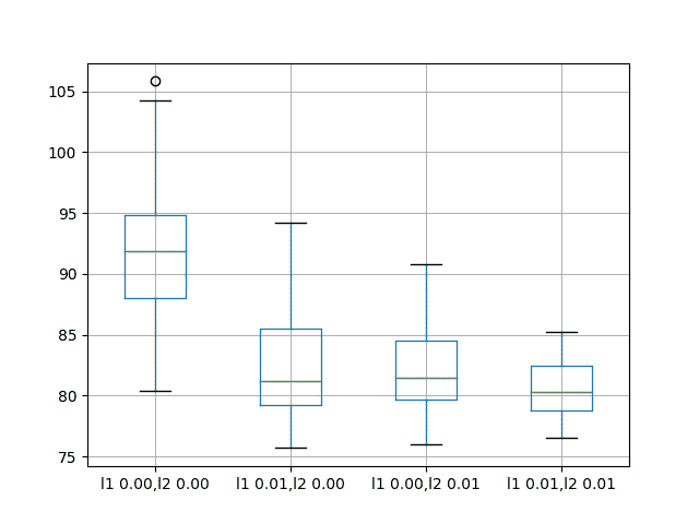  洗發水銷售數據集中輸入重量正規化表現的盒子和晶須圖 ## 復發性體重正則化 最后，我們還可以將正則化應用于每個 LSTM 單元上的循環連接。 在 Keras 中，這是通過將 _recurrent_regularizer_ 參數設置為正則化類來實現的。 我們將測試與前一節中使用的相同的正則化器配置，具體為： * L1L2（0.0,0.0）[例如基線] * L1L2（0.01,0.0）[例如 L1] * L1L2（0.0,0.01）[例如 L2] * L1L2（0.01,0.01）[例如 L1L2 或彈性網] 下面列出了更新的 _fit_lstm（）_，_ 實驗（）_ 和 _run（）_ 函數，用于使用 LSTM 的偏置權重正則化。 ```py # fit an LSTM network to training data def fit_lstm(train, n_batch, nb_epoch, n_neurons, reg): X, y = train[:, 0:-1], train[:, -1] X = X.reshape(X.shape[0], 1, X.shape[1]) model = Sequential() model.add(LSTM(n_neurons, batch_input_shape=(n_batch, X.shape[1], X.shape[2]), stateful=True, recurrent_regularizer=reg)) model.add(Dense(1)) model.compile(loss='mean_squared_error', optimizer='adam') for i in range(nb_epoch): model.fit(X, y, epochs=1, batch_size=n_batch, verbose=0, shuffle=False) model.reset_states() return model # run a repeated experiment def experiment(series, n_lag, n_repeats, n_epochs, n_batch, n_neurons, reg): # transform data to be stationary raw_values = series.values diff_values = difference(raw_values, 1) # transform data to be supervised learning supervised = timeseries_to_supervised(diff_values, n_lag) supervised_values = supervised.values[n_lag:,:] # split data into train and test-sets train, test = supervised_values[0:-12], supervised_values[-12:] # transform the scale of the data scaler, train_scaled, test_scaled = scale(train, test) # run experiment error_scores = list() for r in range(n_repeats): # fit the model train_trimmed = train_scaled[2:, :] lstm_model = fit_lstm(train_trimmed, n_batch, n_epochs, n_neurons, reg) # forecast test dataset test_reshaped = test_scaled[:,0:-1] test_reshaped = test_reshaped.reshape(len(test_reshaped), 1, 1) output = lstm_model.predict(test_reshaped, batch_size=n_batch) predictions = list() for i in range(len(output)): yhat = output[i,0] X = test_scaled[i, 0:-1] # invert scaling yhat = invert_scale(scaler, X, yhat) # invert differencing yhat = inverse_difference(raw_values, yhat, len(test_scaled)+1-i) # store forecast predictions.append(yhat) # report performance rmse = sqrt(mean_squared_error(raw_values[-12:], predictions)) print('%d) Test RMSE: %.3f' % (r+1, rmse)) error_scores.append(rmse) return error_scores # configure the experiment def run(): # load dataset series = read_csv('shampoo-sales.csv', header=0, parse_dates=[0], index_col=0, squeeze=True, date_parser=parser) # configure the experiment n_lag = 1 n_repeats = 30 n_epochs = 1000 n_batch = 4 n_neurons = 3 regularizers = [L1L2(l1=0.0, l2=0.0), L1L2(l1=0.01, l2=0.0), L1L2(l1=0.0, l2=0.01), L1L2(l1=0.01, l2=0.01)] # run the experiment results = DataFrame() for reg in regularizers: name = ('l1 %.2f,l2 %.2f' % (reg.l1, reg.l2)) results[name] = experiment(series, n_lag, n_repeats, n_epochs, n_batch, n_neurons, reg) # summarize results print(results.describe()) # save boxplot results.boxplot() pyplot.savefig('experiment_reg_recurrent.png') ``` 運行此實驗會打印每個已評估配置的描述性統計信息。 結果表明，對 LSTM 的復發連接使用正則化對此問題沒有明顯的好處。 嘗試的所有變化的平均表現導致比基線模型更差的表現。 ```py l1 0.00,l2 0.00 l1 0.01,l2 0.00 l1 0.00,l2 0.01 l1 0.01,l2 0.01 count 30.000000 30.000000 30.000000 30.000000 mean 92.918797 100.675386 101.302169 96.820026 std 7.172764 3.866547 5.228815 3.966710 min 72.967841 93.789854 91.063592 89.367600 25% 90.311185 98.014045 98.222732 94.787647 50% 92.327824 100.546756 101.903350 95.727549 75% 95.989761 103.491192 104.918266 98.240613 max 110.529422 108.788604 110.712064 111.185747 ``` 還會創建一個框和胡須圖來比較每個配置的結果分布。 該圖顯示了與摘要統計相同的故事，表明使用復發體重正則化幾乎沒有益處。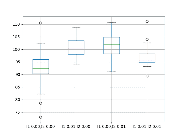  洗發水銷售數據集中復發重量正常化的盒子和晶須圖 ## 擴展 本節列出了后續實驗的想法，以擴展本教程中的工作。 * **輸入權重正則化**。輸入權重正則化對該問題的實驗結果表明了上市績效的巨大希望。這可以通過網格搜索不同的 L1 和 L2 值來進一步研究，以找到最佳配置。 * **行為動態**。可以通過在訓練時期上繪制訓練和測試 RMSE 來研究每個權重正則化方案的動態行為，以獲得對過度擬合或欠擬合行為模式的權重正則化的想法。 * **結合正則化**。可以設計實驗來探索組合不同重量正則化方案的效果。 * **激活正則化**。 Keras 還支持激活正則化，這可能是探索對 LSTM 施加約束并減少過度擬合的另一種途徑。 ## 摘要 在本教程中，您了解了如何將權重正則化與 LSTM 一起用于時間序列預測。 具體來說，你學到了： * 如何設計一個強大的測試工具來評估 LSTM 網絡的時間序列預測。 * 如何在 LSTM 上配置偏差權重正則化用于時間序列預測。 * 如何在 LSTM 上配置輸入和循環權重正則化以進行時間序列預測。 您對使用 LSTM 網絡的權重正則化有任何疑問嗎？ 在下面的評論中提出您的問題，我會盡力回答。