# Python 中概率評分方法的簡要介紹 > 原文： [https://machinelearningmastery.com/how-to-score-probability-predictions-in-python/](https://machinelearningmastery.com/how-to-score-probability-predictions-in-python/) #### 如何評估 Python 中的概率預測和 為不同的度量標準開發直覺。 為分類問題預測概率而不是類標簽可以為預測提供額外的細微差別和不確定性。 增加的細微差別允許使用更復雜的度量來解釋和評估預測的概率。通常，用于評估預測概率的準確性的方法被稱為[評分規則](https://en.wikipedia.org/wiki/Scoring_rule)或評分函數。 在本教程中，您將發現三種評分方法，可用于評估分類預測建模問題的預測概率。 完成本教程后，您將了解： * 對數損失得分嚴重影響遠離其預期值的預測概率。 * Brier 得分比對數損失更溫和，但仍與預期值的距離成比例。 * ROC 曲線下的區域總結了模型預測真陽性病例的概率高于真陰性病例的可能性。 讓我們開始吧。 * **更新 Sept / 2018** ：修正了 AUC 無技能的描述。  Python 中概率評分方法的簡要介紹 [Paul Balfe](https://www.flickr.com/photos/paul_e_balfe/39642542840/) 的照片，保留一些權利。 ## 教程概述 本教程分為四個部分;他們是： 1. 記錄損失分數 2. 布里爾得分 3. ROC AUC 得分 4. 調整預測概率 ## 記錄損失分數 對數損失，也稱為“邏輯損失”，“對數損失”或“交叉熵”可以用作評估預測概率的度量。 將每個預測概率與實際類輸出值（0 或 1）進行比較，并計算基于與預期值的距離來懲罰概率的分數。罰分為對數，小差異（0.1 或 0.2）得分較小，差異較大（0.9 或 1.0）。 具有完美技能的模型具有 0.0 的對數損失分數。 為了總結使用對數損失的模型的技能，計算每個預測概率的對數損失，并報告平均損失。 可以使用 scikit-learn 中的 [log_loss（）](http://scikit-learn.org/stable/modules/generated/sklearn.metrics.log_loss.html)函數在 Python 中實現日志丟失。 例如： ``` from sklearn.metrics import log_loss ... model = ... testX, testy = ... # predict probabilities probs = model.predict_proba(testX) # keep the predictions for class 1 only probs = probs[:, 1] # calculate log loss loss = log_loss(testy, probs) ``` 在二元分類案例中，函數將真實結果值列表和概率列表作為參數，并計算預測的平均對數損失。 我們可以通過一個例子來制作單一的對數損失分數。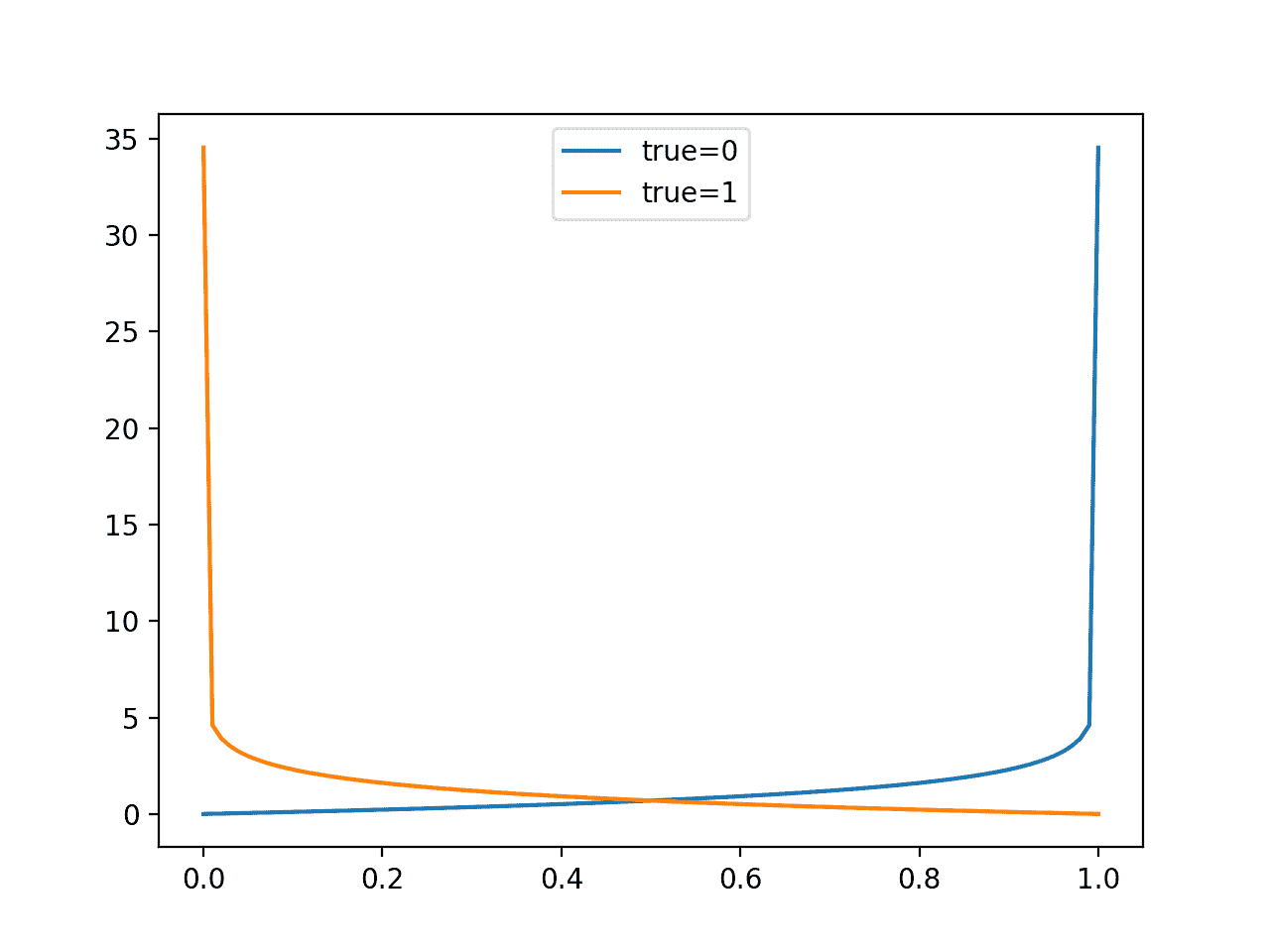 給定 0 的特定已知結果，我們可以以 0.01 增量（101 個預測）預測 0.0 到 1.0 的值，并計算每個的對數損失。結果是曲線顯示每個預測在概率遠離預期值時受到多少懲罰。我們可以對已知的 1 結果重復此操作，并反過來看相同的曲線。 下面列出了完整的示例。 ``` # plot impact of logloss for single forecasts from sklearn.metrics import log_loss from matplotlib import pyplot from numpy import array # predictions as 0 to 1 in 0.01 increments yhat = [x*0.01 for x in range(0, 101)] # evaluate predictions for a 0 true value losses_0 = [log_loss([0], [x], labels=[0,1]) for x in yhat] # evaluate predictions for a 1 true value losses_1 = [log_loss([1], [x], labels=[0,1]) for x in yhat] # plot input to loss pyplot.plot(yhat, losses_0, label='true=0') pyplot.plot(yhat, losses_1, label='true=1') pyplot.legend() pyplot.show() ``` 運行該示例會創建一個折線圖，顯示真實標簽為 0 和 1 的情況下概率預測的損失分數從 0.0 到 1.0。 這有助于建立對評估預測時損失分數的影響的直覺。  具有對數損失的評估預測線圖 模型技能被報告為測試數據集中預測的平均對數損失。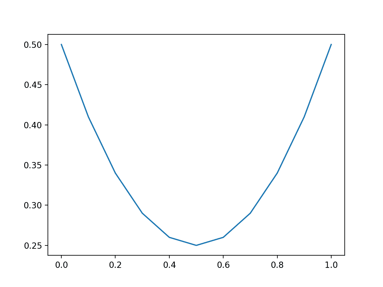 平均而言，當測試集中兩個類之間存在較大的不平衡時，我們可以預期得分將適用于平衡數據集并具有誤導性。這是因為預測 0 或小概率將導致小的損失。 我們可以通過比較損失值的分布來預測平衡和不平衡數據集的不同常數概率來證明這一點。 首先，對于 50 個 0 級和 1 級示例的平衡數據集，下面的示例以 0.1 為增量預測值為 0.0 到 1.0。 ``` # plot impact of logloss with balanced datasets from sklearn.metrics import log_loss from matplotlib import pyplot from numpy import array # define an imbalanced dataset testy = [0 for x in range(50)] + [1 for x in range(50)] # loss for predicting different fixed probability values predictions = [0.0, 0.1, 0.2, 0.3, 0.4, 0.5, 0.6, 0.7, 0.8, 0.9, 1.0] losses = [log_loss(testy, [y for x in range(len(testy))]) for y in predictions] # plot predictions vs loss pyplot.plot(predictions, losses) pyplot.show() ``` 運行該示例，我們可以看到模型更好地預測不尖銳（靠近邊緣）并回到分布中間的概率值。 錯誤概率的懲罰是非常大的。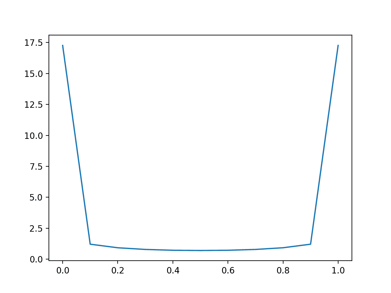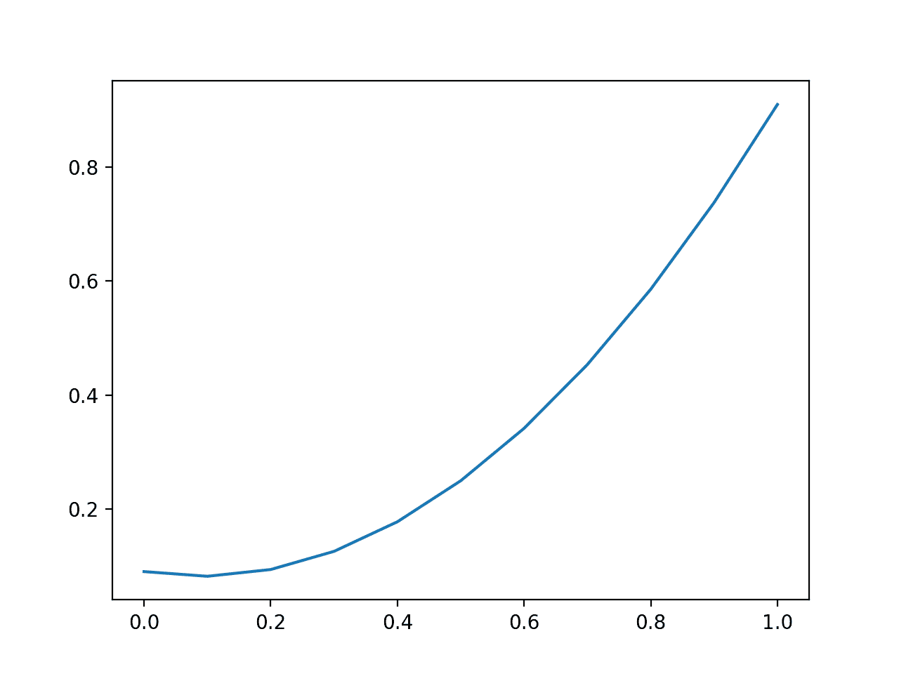  預測平衡數據集對數損失的線圖 我們可以使用不平衡的數據集重復此實驗，其中 0 級到 1 級的比率為 10：1。 ``` # plot impact of logloss with imbalanced datasets from sklearn.metrics import log_loss from matplotlib import pyplot from numpy import array # define an imbalanced dataset testy = [0 for x in range(100)] + [1 for x in range(10)] # loss for predicting different fixed probability values predictions = [0.0, 0.1, 0.2, 0.3, 0.4, 0.5, 0.6, 0.7, 0.8, 0.9, 1.0] losses = [log_loss(testy, [y for x in range(len(testy))]) for y in predictions] # plot predictions vs loss pyplot.plot(predictions, losses) pyplot.show() ``` 在這里，我們可以看到，傾向于預測非常小的概率的模型將表現良好，樂觀地如此。 預測 0.1 的恒定概率的幼稚模型將是要擊敗的基線模型。 結果表明，在不平衡數據集的情況下，應該仔細解釋用對數損失評估的模型技能，可能相對于數據集中第 1 類的基本速率進行調整。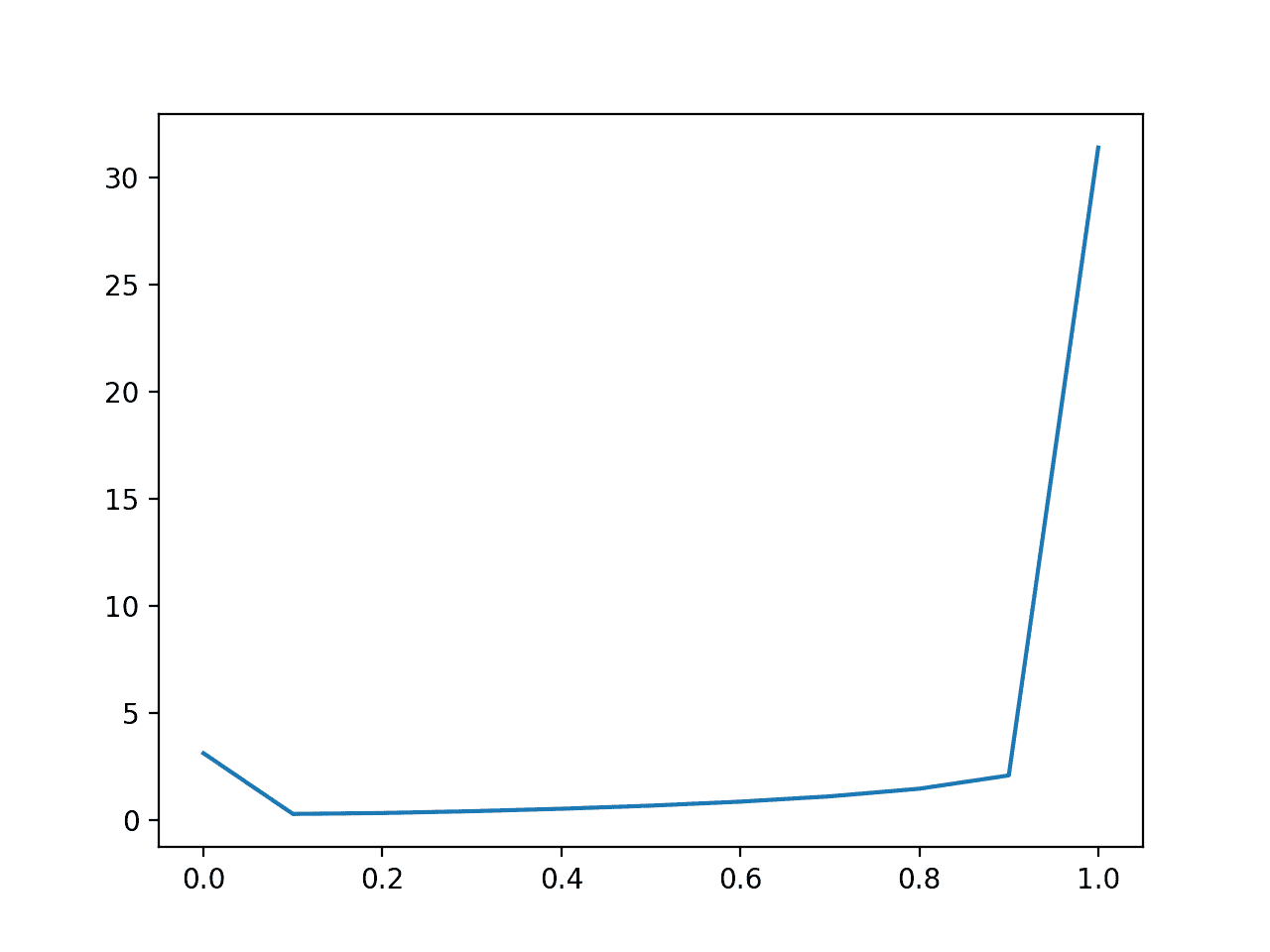  預測不平衡數據集的對數損失的線圖 ## 布里爾得分 以格倫布里爾命名的布里爾分數計算預測概率與預期值之間的均方誤差。 該分數總結了概率預測中的誤差幅度。 錯誤分數始終介于 0.0 和 1.0 之間，其中具有完美技能的模型得分為 0.0。 遠離預期概率的預測會受到懲罰，但與對數丟失的情況相比會受到嚴重影響。 模型的技能可以概括為針對測試數據集預測的所有概率的平均 Brier 分數。 可以使用 scikit-learn 中的 [brier_score_loss（）函數](http://scikit-learn.org/stable/modules/generated/sklearn.metrics.brier_score_loss.html)在 Python 中計算 Brier 分數。它將測試數據集中所有示例的真實類值（0,1）和預測概率作為參數，并返回平均 Brier 分數。 For example: ``` from sklearn.metrics import brier_score_loss ... model = ... testX, testy = ... # predict probabilities probs = model.predict_proba(testX) # keep the predictions for class 1 only probs = probs[:, 1] # calculate bier score loss = brier_score_loss(testy, probs) ``` 我們可以通過比較單個概率預測的 Brier 得分來評估預測誤差的影響，將誤差從 0.0 增加到 1.0。 The complete example is listed below. ``` # plot impact of brier for single forecasts from sklearn.metrics import brier_score_loss from matplotlib import pyplot from numpy import array # predictions as 0 to 1 in 0.01 increments yhat = [x*0.01 for x in range(0, 101)] # evaluate predictions for a 1 true value losses = [brier_score_loss([1], [x], pos_label=[1]) for x in yhat] # plot input to loss pyplot.plot(yhat, losses) pyplot.show() ``` 運行該示例創建概率預測誤差的絕對值（x 軸）與計算的 Brier 分數（y 軸）的關系圖。 我們可以看到熟悉的二次曲線，從 0 到 1，誤差平方。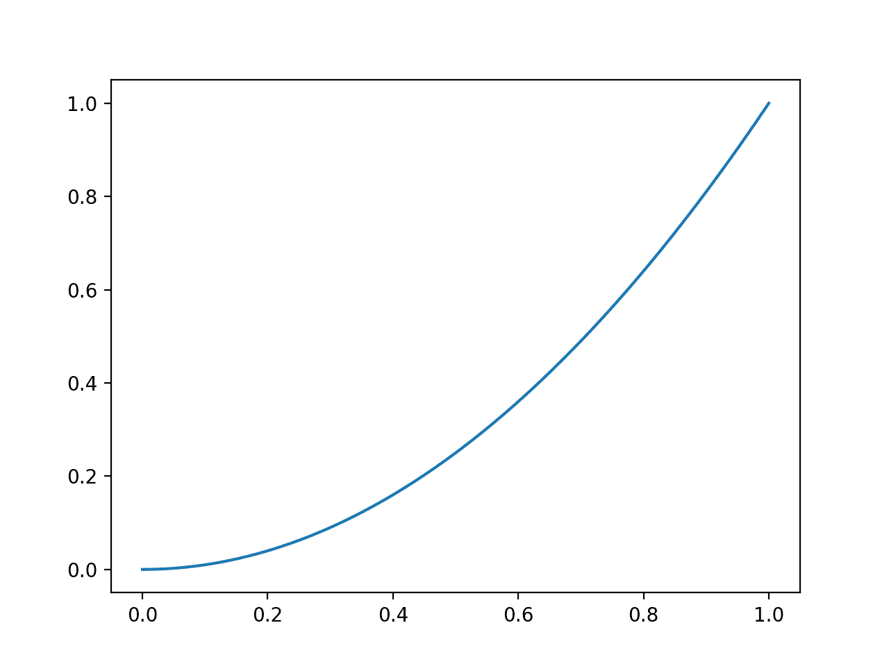  用 Brier 評分評估預測的線圖 模型技能被報告為測試數據集中預測的平均 Brier。 與對數丟失一樣，當測試集中兩個類之間存在較大的不平衡時，我們可以預期得分將適用于平衡數據集并具有誤導性。 We can demonstrate this by comparing the distribution of loss values when predicting different constant probabilities for a balanced and an imbalanced dataset. First, the example below predicts values from 0.0 to 1.0 in 0.1 increments for a balanced dataset of 50 examples of class 0 and 1. ``` # plot impact of brier score with balanced datasets from sklearn.metrics import brier_score_loss from matplotlib import pyplot from numpy import array # define an imbalanced dataset testy = [0 for x in range(50)] + [1 for x in range(50)] # brier score for predicting different fixed probability values predictions = [0.0, 0.1, 0.2, 0.3, 0.4, 0.5, 0.6, 0.7, 0.8, 0.9, 1.0] losses = [brier_score_loss(testy, [y for x in range(len(testy))]) for y in predictions] # plot predictions vs loss pyplot.plot(predictions, losses) pyplot.show() ``` 運行這個例子，我們可以看到一個模型更好地預測道路概率值的中間值，如 0.5。 與對于緊密概率非常平坦的對數損失不同，拋物線形狀顯示隨著誤差增加而得分懲罰的明顯二次增加。  平衡數據集預測 Brier 分數的線圖 We can repeat this experiment with an imbalanced dataset with a 10:1 ratio of class 0 to class 1. ``` # plot impact of brier score with imbalanced datasets from sklearn.metrics import brier_score_loss from matplotlib import pyplot from numpy import array # define an imbalanced dataset testy = [0 for x in range(100)] + [1 for x in range(10)] # brier score for predicting different fixed probability values predictions = [0.0, 0.1, 0.2, 0.3, 0.4, 0.5, 0.6, 0.7, 0.8, 0.9, 1.0] losses = [brier_score_loss(testy, [y for x in range(len(testy))]) for y in predictions] # plot predictions vs loss pyplot.plot(predictions, losses) pyplot.show() ``` 運行該示例，我們看到不平衡數據集的圖片非常不同。 與平均對數損失一樣，平均 Brier 分數將在不平衡數據集上呈現樂觀分數，獎勵小預測值，從而減少大多數類別的錯誤。 在這些情況下，Brier 分數應該相對于幼稚預測（例如少數類的基本率或上例中的 0.1）進行比較，或者通過樸素分數進行歸一化。 后一個例子很常見，稱為 Brier 技能分數（BSS）。 ``` BSS = 1 - (BS / BS_ref) ``` 其中 BS 是模型的 Brier 技能，而 BS_ref 是樸素預測的 Brier 技能。 Brier 技能分數報告了概率預測相對于樸素預測的相對技能。 對 scikit-learn API 的一個很好的更新是將參數添加到 _brier_score_loss（）_ 以支持 Brier 技能分數的計算。  不平衡數據集預測 Brier 分數的線圖 ## ROC AUC 得分 二進制（兩級）分類問題的預測概率可以用閾值來解釋。 閾值定義概率映射到 0 級與 1 級的點，其中默認閾值為 0.5。替代閾值允許模型針對更高或更低的誤報和漏報進行調整。 操作員調整閾值對于一種類型的錯誤或多或少比另一種錯誤或者模型不成比例地或多或少地具有特定類型的錯誤的問題尤為重要。 接收器操作特性或 ROC 曲線是對于多個閾值在 0.0 和 1.0 之間的模型的預測的真陽性率與假陽性率的曲線圖。 在從左下角到右上角的圖的對角線上繪制對于給定閾值沒有技能的預測。此行表示每個閾值的無技能預測。 具有技能的模型在該對角線上方具有向左上角彎曲的曲線。 下面是在二元分類問題上擬合邏輯回歸模型并計算和繪制 500 個新數據實例的測試集上的預測概率的 ROC 曲線的示例。 ``` # roc curve from sklearn.datasets import make_classification from sklearn.linear_model import LogisticRegression from sklearn.model_selection import train_test_split from sklearn.metrics import roc_curve from matplotlib import pyplot # generate 2 class dataset X, y = make_classification(n_samples=1000, n_classes=2, random_state=1) # split into train/test sets trainX, testX, trainy, testy = train_test_split(X, y, test_size=0.5, random_state=2) # fit a model model = LogisticRegression() model.fit(trainX, trainy) # predict probabilities probs = model.predict_proba(testX) # keep probabilities for the positive outcome only probs = probs[:, 1] # calculate roc curve fpr, tpr, thresholds = roc_curve(testy, probs) # plot no skill pyplot.plot([0, 1], [0, 1], linestyle='--') # plot the roc curve for the model pyplot.plot(fpr, tpr) # show the plot pyplot.show() ``` 運行該示例創建了一個 ROC 曲線示例，可以與主對角線上的無技能線進行比較。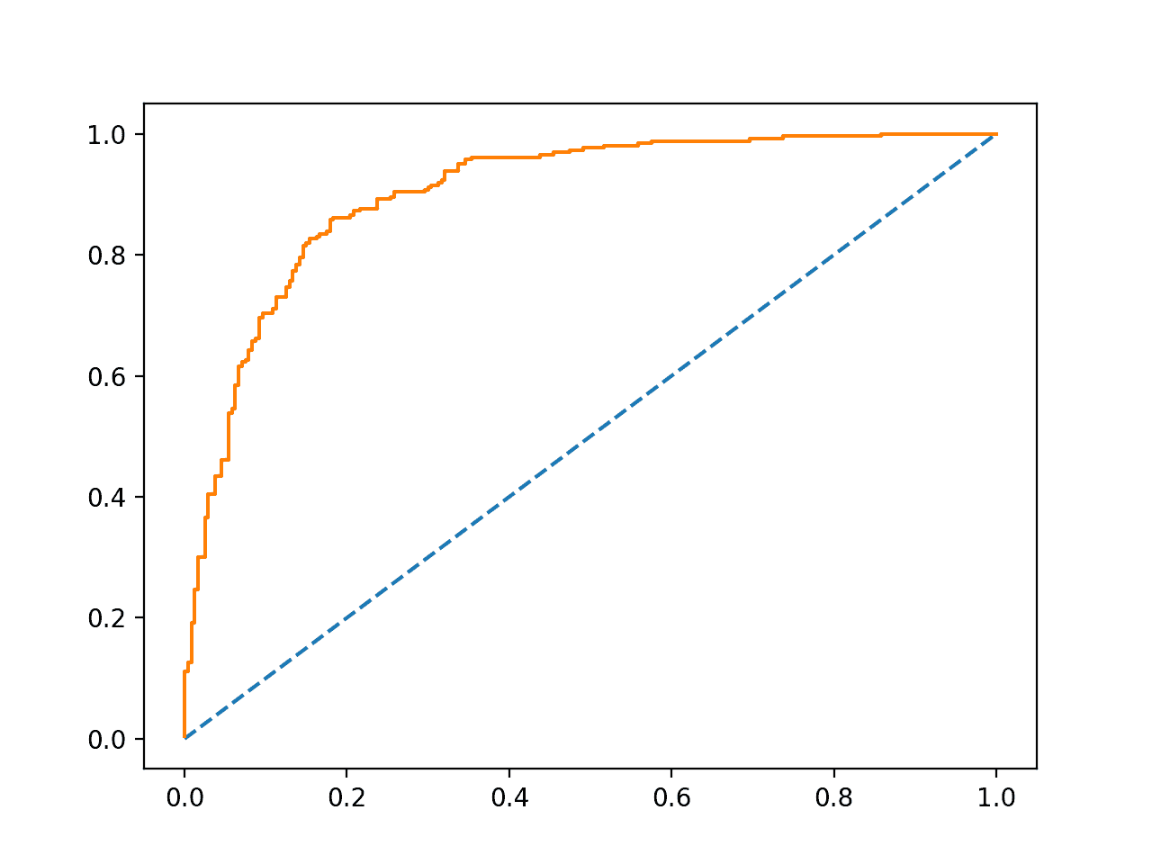  示例 ROC 曲線 ROC 曲線下的綜合區域稱為 AUC 或 ROC AUC，可以衡量所有評估閾值的模型技能。 AUC 得分為 0.5 表明沒有技能，例如沿著對角線的曲線，而 AUC 為 1.0 表示完美技能，所有點沿著左側 y 軸和頂部 x 軸朝向左上角。 AUC 為 0.0 表明完全不正確的預測。 具有較大面積的模型的預測在閾值上具有更好的技能，盡管模型之間的曲線的特定形狀將變化，可能提供通過預先選擇的閾值來優化模型的機會。通常，在準備好模型之后，操作員選擇閾值。 可以使用 scikit-learn 中的 [roc_auc_score（）函數](http://scikit-learn.org/stable/modules/generated/sklearn.calibration.calibration_curve.html)在 Python 中計算 AUC。 此函數將真實輸出值和預測概率列表作為參數，并返回 ROC AUC。 For example: ``` from sklearn.metrics import roc_auc_score ... model = ... testX, testy = ... # predict probabilities probs = model.predict_proba(testX) # keep the predictions for class 1 only probs = probs[:, 1] # calculate log loss loss = roc_auc_score(testy, probs) ``` AUC 分數是產生預測的模型將隨機選擇的正例高于隨機選擇的負例的可能性的度量。具體而言，真實事件（class = 1）的概率高于真實的非事件（class = 0）。 這是一個有用的定義，它提供了兩個重要的直覺： * **樸素預測**。 ROC AUC 下的樸素預測是任何恒定概率。如果對每個例子預測相同的概率，則在正面和負面情況之間沒有區別，因此該模型沒有技能（AUC = 0.5）。 * **對類不平衡的不敏感性**。 ROC AUC 是關于模型在不同閾值之間正確區分單個示例的能力的總結。因此，它不關心每個類的基本可能性。 下面，更新演示 ROC 曲線的示例以計算和顯示 AUC。 ``` # roc auc from sklearn.datasets import make_classification from sklearn.linear_model import LogisticRegression from sklearn.model_selection import train_test_split from sklearn.metrics import roc_auc_score from matplotlib import pyplot # generate 2 class dataset X, y = make_classification(n_samples=1000, n_classes=2, random_state=1) # split into train/test sets trainX, testX, trainy, testy = train_test_split(X, y, test_size=0.5, random_state=2) # fit a model model = LogisticRegression() model.fit(trainX, trainy) # predict probabilities probs = model.predict_proba(testX) # keep probabilities for the positive outcome only probs = probs[:, 1] # calculate roc auc auc = roc_auc_score(testy, probs) print(auc) ``` 運行該示例計算并打印在 500 個新示例上評估的邏輯回歸模型的 ROC AUC。 ``` 0.9028044871794871 ``` 選擇 ROC AUC 的一個重要考慮因素是它沒有總結模型的具體判別能力，而是所有閾值的一般判別能力。 它可能是模型選擇的更好工具，而不是量化模型預測概率的實際技能。 ## 調整預測概率 可以調整預測概率以改進甚至游戲表現測量。 例如，對數損失和 Brier 分數量化概率中的平均誤差量。因此，可以通過以下幾種方式調整預測概率以改善這些分數： * **使概率不那么尖銳（不太自信）**。這意味著調整預測概率遠離硬 0 和 1 界限，以限制完全錯誤處罰的影響。 * **將分布轉移到幼稚預測（基準率）**。這意味著將預測概率的平均值轉換為基本概率的概率，例如對于平衡預測問題的 0.5。 通常，使用諸如可靠性圖之類的工具來審查概率的校準可能是有用的。這可以使用 scikit-learn 中的 [calibration_curve（）函數](http://scikit-learn.org/stable/modules/generated/sklearn.calibration.calibration_curve.html)來實現。 某些算法（如 SVM 和神經網絡）可能無法本地預測校準概率。在這些情況下，可以校準概率，進而可以改善所選擇的度量。可以使用 [CalibratedClassifierCV](http://scikit-learn.org/stable/modules/generated/sklearn.calibration.CalibratedClassifierCV.html) 類在 scikit-learn 中校準分類器。 ## 進一步閱讀 如果您希望深入了解，本節將提供有關該主題的更多資源。 ### API * [sklearn.metrics.log_loss API](http://scikit-learn.org/stable/modules/generated/sklearn.metrics.log_loss.html) * [sklearn.metrics.brier_score_loss API](http://scikit-learn.org/stable/modules/generated/sklearn.metrics.brier_score_loss.html) * [sklearn.metrics.roc_curve API](http://scikit-learn.org/stable/modules/generated/sklearn.metrics.roc_curve.html) * [sklearn.metrics.roc_auc_score API](http://scikit-learn.org/stable/modules/generated/sklearn.metrics.roc_auc_score.html) * [sklearn.calibration.calibration_curve API](http://scikit-learn.org/stable/modules/generated/sklearn.calibration.calibration_curve.html) * [sklearn.calibration.CalibratedClassifierCV API](http://scikit-learn.org/stable/modules/generated/sklearn.calibration.CalibratedClassifierCV.html) ### 用品 * [評分規則，維基百科](https://en.wikipedia.org/wiki/Scoring_rule) * [交叉熵，維基百科](https://en.wikipedia.org/wiki/Cross_entropy) * [Log Loss，fast.ai](http://wiki.fast.ai/index.php/Log_Loss) * [Brier 得分，維基百科](https://en.wikipedia.org/wiki/Brier_score) * [接收器操作特性，維基百科](https://en.wikipedia.org/wiki/Receiver_operating_characteristic) ## 摘要 在本教程中，您發現了三個度量標準，可用于評估分類預測建模問題的預測概率。 具體來說，你學到了： * 對數損失得分嚴重影響遠離其預期值的預測概率。 * Brier 得分比對數損失更溫和，但仍與預期值的距離成比例 * ROC 曲線下的區域總結了模型預測真陽性病例的概率高于真陰性病例的可能性。 你有任何問題嗎？ 在下面的評論中提出您的問題，我會盡力回答。