# 嶺正則化 以下是嶺正則化回歸的完整代碼，用于訓練模型以預測波士頓房屋定價： ```py num_outputs = y_train.shape[1] num_inputs = X_train.shape[1] x_tensor = tf.placeholder(dtype=tf.float32, shape=[None, num_inputs], name='x') y_tensor = tf.placeholder(dtype=tf.float32, shape=[None, num_outputs], name='y') w = tf.Variable(tf.zeros([num_inputs, num_outputs]), dtype=tf.float32, name='w') b = tf.Variable(tf.zeros([num_outputs]), dtype=tf.float32, name='b') model = tf.matmul(x_tensor, w) + b ridge_param = tf.Variable(0.8, dtype=tf.float32) ridge_loss = tf.reduce_mean(tf.square(w)) * ridge_param loss = tf.reduce_mean(tf.square(model - y_tensor)) + ridge_loss learning_rate = 0.001 optimizer = tf.train.GradientDescentOptimizer(learning_rate).minimize(loss) mse = tf.reduce_mean(tf.square(model - y_tensor)) y_mean = tf.reduce_mean(y_tensor) total_error = tf.reduce_sum(tf.square(y_tensor - y_mean)) unexplained_error = tf.reduce_sum(tf.square(y_tensor - model)) rs = 1 - tf.div(unexplained_error, total_error) num_epochs = 1500 loss_epochs = np.empty(shape=[num_epochs],dtype=np.float32) mse_epochs = np.empty(shape=[num_epochs],dtype=np.float32) rs_epochs = np.empty(shape=[num_epochs],dtype=np.float32) mse_score = 0.0 rs_score = 0.0 with tf.Session() as tfs: tfs.run(tf.global_variables_initializer()) for epoch in range(num_epochs): feed_dict = {x_tensor: X_train, y_tensor: y_train} loss_val, _ = tfs.run([loss, optimizer], feed_dict=feed_dict) loss_epochs[epoch] = loss_val feed_dict = {x_tensor: X_test, y_tensor: y_test} mse_score, rs_score = tfs.run([mse, rs], feed_dict=feed_dict) mse_epochs[epoch] = mse_score rs_epochs[epoch] = rs_score print('For test data : MSE = {0:.8f}, R2 = {1:.8f} '.format( mse_score, rs_score)) ``` 我們得到以下結果： ```py 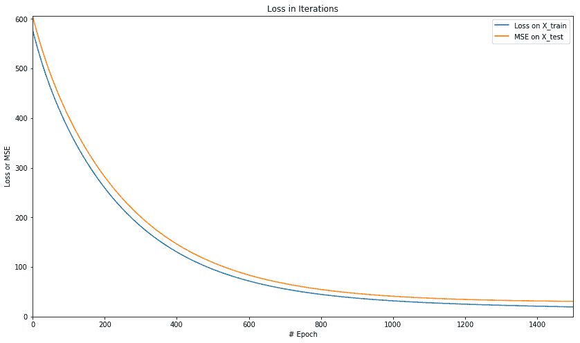For test data : MSE = 30.64177132, R2 = 0.63988018 ``` 繪制損失和 MSE 的值，我們得到以下損失圖：  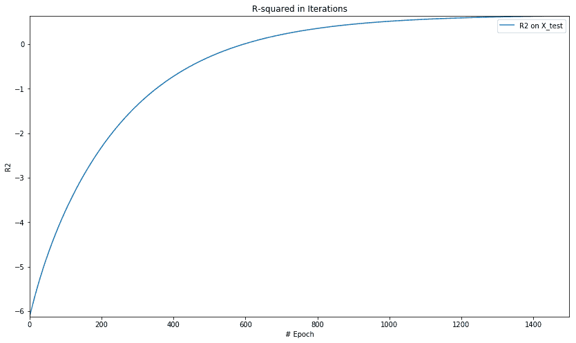我們得到以下 R 平方圖：  讓我們來看看套索和嶺正則化方法的組合。