## 10.2 效果大小 > “統計顯著性是最不有趣的結果。你應該用數量尺度來描述結果——不僅僅是治療對人有影響，還有它對人有多大的影響。”基因玻璃（Ref） 在最后一章中，我們討論了統計學意義不一定反映實際意義的觀點。為了討論實際意義，我們需要一種標準的方法來根據實際數據描述效應的大小，我們稱之為 _ 效應大小 _。在本節中，我們將介紹這個概念，并討論計算影響大小的各種方法。 效應大小是一種標準化的測量，它將某些統計效應的大小與參考量（如統計的可變性）進行比較。在一些科學和工程領域中，這個概念被稱為“信噪比”。有許多不同的方法可以量化效果大小，這取決于數據的性質。 ### 10.2.1 科恩 影響大小最常見的度量之一是以統計學家雅各布·科恩（Jacob Cohen）的名字命名的 _ 科恩的 D_，他在 1994 年發表的題為“地球是圓的（P&lt；.05）”的論文中最為著名。它用于量化兩種方法之間的差異，根據它們的標準偏差：  其中和是兩組的平均值，而是合并標準偏差（這是兩個樣本的標準偏差的組合，由樣本大小加權）：  其中和是樣品尺寸，和分別是兩組的標準偏差。 有一個常用的尺度可以用科恩的 D 來解釋效應的大小： <colgroup><col style="width: 8%"> <col style="width: 22%"></colgroup> | D | 解釋 | | --- | --- | | 0.2 條 | 小的 | | 0.5 倍 | 中等的 | | 0.8 倍 | 大的 | 觀察一些常見的理解效果，有助于理解這些解釋。 ```r # compute effect size for gender difference in NHANES NHANES_sample <- NHANES_adult %>% drop_na(Height) %>% sample_n(250) hsum <- NHANES_sample %>% group_by(Gender) %>% summarize( meanHeight = mean(Height), varHeight = var(Height), n = n() ) #pooled SD s_height_gender <- sqrt( ((hsum$n[1] - 1) * hsum$varHeight[1] + (hsum$n[2] - 1) * hsum$varHeight[2]) / (hsum$n[1] + hsum$n[2] - 2) ) #cohen's d d_height_gender <- (hsum$meanHeight[2] - hsum$meanHeight[1]) / s_height_gender sprintf("Cohens d for male vs. female height = %0.2f", d_height_gender) ``` ```r ## [1] "Cohens d for male vs. female height = 1.95" ``` 參照上表，身高性別差異的影響大小（d=1.95）很大。我們也可以通過觀察樣本中男性和女性身高的分布來看到這一點。圖[10.2](#fig:genderHist)顯示，這兩個分布雖然仍然重疊，但分離得很好，突出了這樣一個事實：即使兩個組之間的差異有很大的影響大小，每個組中的個體也會更像另一個組。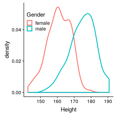  圖 10.2 nhanes 數據集中男性和女性身高的平滑柱狀圖，顯示了明顯不同但明顯重疊的分布。 同樣值得注意的是，我們很少在科學中遇到這種規模的影響，部分原因是它們是如此明顯的影響，以至于我們不需要科學研究來找到它們。正如我們將在第[17](#doing-reproducible-research)章中看到的那樣，在科學研究中報告的非常大的影響往往反映出有問題的研究實踐的使用，而不是自然界中真正的巨大影響。同樣值得注意的是，即使有如此巨大的影響，這兩種分布仍然是重疊的——會有一些女性比普通男性高，反之亦然。對于最有趣的科學效應來說，重疊的程度會大得多，所以我們不應該馬上就基于一個大的效應大小得出關于不同人群的強有力的結論。 ### 10.2.2 皮爾遜 R Pearson 的 _r_ 也稱為 _ 相關系數 _，是對兩個連續變量之間線性關系強度的度量。我們將在[13](#modeling-continuous-relationships)章中更詳細地討論相關性，因此我們將保存該章的詳細信息；這里，我們簡單地介紹 _r_ 作為量化兩個變量之間關系的方法。 _r_ 是一個在-1 到 1 之間變化的度量值，其中值 1 表示變量之間的完全正關系，0 表示沒有關系，而-1 表示完全負關系。圖[10.3](#fig:corrFig)顯示了使用隨機生成的數據的各種相關級別的示例。  圖 10.3 不同水平皮爾遜 R 的示例。 ### 10.2.3 優勢比 在我們之前關于概率的討論中，我們討論了概率的概念——也就是說，某些事件發生與未發生的相對可能性：  優勢比只是兩個優勢比。例如，讓我們以吸煙和肺癌為例。2012 年發表在《國際癌癥雜志》上的一項研究（Pesch 等人 2012 年）關于吸煙者和從未吸煙的個體肺癌發生率的綜合數據，通過許多不同的研究。請注意，這些數據來自病例對照研究，這意味著這些研究的參與者之所以被招募，是因為他們要么患了癌癥，要么沒有患癌癥；然后檢查他們的吸煙狀況。因此，這些數字并不代表一般人群中吸煙者的癌癥患病率，但它們可以告訴我們癌癥與吸煙之間的關系。 ```r # create table for cancer occurrence depending on smoking status smokingDf <- tibble( NeverSmoked = c(2883, 220), CurrentSmoker = c(3829, 6784), row.names = c("NoCancer", "Cancer") ) pander(smokingDf) ``` <colgroup><col style="width: 19%"> <col style="width: 22%"> <col style="width: 15%"></colgroup> | 從不吸煙 | 當前吸煙者 | 行名稱 | | --- | --- | --- | | 2883 個 | 3829 年 | 無癌癥者 | | 220 | 6784 個 | 癌癥 | 我們可以將這些數字轉換為每個組的優勢比： ```r # convert smoking data to odds smokingDf <- smokingDf %>% mutate( pNeverSmoked = NeverSmoked / sum(NeverSmoked), pCurrentSmoker = CurrentSmoker / sum(CurrentSmoker) ) oddsCancerNeverSmoked <- smokingDf$NeverSmoked[2] / smokingDf$NeverSmoked[1] oddsCancerCurrentSmoker <- smokingDf$CurrentSmoker[2] / smokingDf$CurrentSmoker[1] ``` 從未吸煙的人患肺癌的幾率為 0.08，而目前吸煙者患肺癌的幾率為 1.77。這些比值告訴我們兩組患者患癌癥的相對可能性： ```r #compute odds ratio oddsRatio <- oddsCancerCurrentSmoker/oddsCancerNeverSmoked sprintf('odds ratio of cancer for smokers vs. nonsmokers: %0.3f',oddsRatio) ``` ```r ## [1] "odds ratio of cancer for smokers vs. nonsmokers: 23.218" ``` 23.22 的比值比告訴我們，吸煙者患癌癥的幾率大約是不吸煙者的 23 倍。