## 11.4 估計后驗分布 在前一個例子中，只有兩種可能的結果——爆炸物要么在那里，要么不在那里——我們想知道給出數據后，哪種結果最有可能。但是，在其他情況下，我們希望使用貝葉斯估計來估計參數的數值。比如說，我們想知道一種新的止痛藥的有效性；為了測試這一點，我們可以給一組病人服用這種藥物，然后詢問他們服用這種藥物后疼痛是否有所改善。我們可以使用貝葉斯分析來估計藥物對誰有效的比例。 ### 11.4.1 規定 在這種情況下，我們沒有任何關于藥物有效性的先驗信息，因此我們將使用 _ 均勻分布 _ 作為先驗值，因為所有值在均勻分布下都是相同的。為了簡化示例，我們將只查看 99 個可能有效性值的子集（從.01 到.99，步驟為.01）。因此，每個可能值的先驗概率為 1/99。 ### 11.4.2 收集一些數據 我們需要一些數據來估計藥物的效果。假設我們給 100 個人用藥，結果如下： ```r # create a table with results nResponders <- 64 nTested <- 100 drugDf <- tibble( outcome = c("improved", "not improved"), number = c(nResponders, nTested - nResponders) ) pander(drugDf) ``` <colgroup><col style="width: 20%"> <col style="width: 11%"></colgroup> | 結果 | 數 | | --- | --- | | 改進 | 64 個 | | 沒有改善 | 36 歲 | ### 11.4.3 計算可能性 我們可以使用 r 中的`dbinom()`函數計算有效性參數的任何特定值下的數據的可能性。在圖[11.1](#fig:like2)中，您可以看到響應器數量對幾個不同值的可能性曲線。從這一點來看，我們觀察到的數據在假設下的可能性相對較大，在假設下的可能性相對較小，在假設下的可能性相對較小。貝葉斯推理的一個基本思想是，我們將試圖找到我們感興趣的參數的值，這使得數據最有可能，同時也考慮到我們的先驗知識。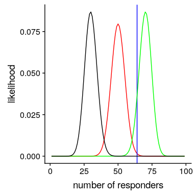  圖 11.1 幾個不同假設下每個可能數量的應答者的可能性（P（應答）=0.5（紅色），0.7（綠色），0.3（黑色）。觀察值以藍色顯示。 ### 11.4.4 計算邊際可能性 除了不同假設下數據的可能性外，我們還需要知道數據的總體可能性，并結合所有假設（即邊際可能性）。這種邊際可能性主要是重要的，因為它有助于確保后驗值是真實概率。在這種情況下，我們使用一組離散的可能參數值使得計算邊際似然變得容易，因為我們只需計算每個假設下每個參數值的似然，并將它們相加。 ```r # compute marginal likelihood likeDf <- likeDf %>% mutate(uniform_prior = array(1 / n())) # multiply each likelihood by prior and add them up marginal_likelihood <- sum( dbinom( x = nResponders, # the number who responded to the drug size = 100, # the number tested likeDf$presp # the likelihood of each response ) * likeDf$uniform_prior ) sprintf("marginal likelihood = %0.4f", marginal_likelihood) ``` ```r ## [1] "marginal likelihood = 0.0100" ``` ### 11.4.5 計算后部 我們現在有了所有需要計算所有可能值的后驗概率分布的部分，如圖[11.2](#fig:posteriorDist)所示。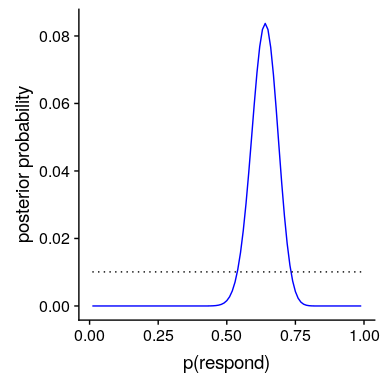 ```r # Create data for use in figure bayesDf <- tibble( steps = seq(from = 0.01, to = 0.99, by = 0.01) ) %>% mutate( likelihoods = dbinom( x = nResponders, size = 100, prob = steps ), priors = dunif(steps) / length(steps), posteriors = (likelihoods * priors) / marginal_likelihood ) ```  圖 11.2 藍色后驗概率分布圖與均勻前驗概率分布圖（黑色虛線）。 ### 11.4.6 最大后驗概率（MAP）估計 根據我們的數據，我們希望獲得樣本的估計值。一種方法是找到后驗概率最高的值，我們稱之為后驗概率（map）估計的 _ 最大值。我們可以從[11.2](#fig:posteriorDist)中的數據中找到：_ ```r # compute MAP estimate MAP_estimate <- bayesDf %>% arrange(desc(posteriors)) %>% slice(1) %>% pull(steps) sprintf("MAP estimate = %0.4f", MAP_estimate) ``` ```r ## [1] "MAP estimate = 0.6400" ``` 請注意，這只是樣本中反應者的比例——這是因為之前的反應是一致的，因此沒有影響我們的反應。 ### 11.4.7 可信區間 通常我們想知道的不僅僅是對后位的單一估計，而是一個我們確信后位下降的間隔。我們之前討論過頻繁推理背景下的置信區間概念，您可能還記得，置信區間的解釋特別復雜。我們真正想要的是一個區間，在這個區間中，我們確信真正的參數會下降，而貝葉斯統計可以給我們一個這樣的區間，我們稱之為 _ 可信區間 _。 在某些情況下，可信區間可以根據已知的分布用數字 _ 計算，但從后驗分布中取樣，然后計算樣本的分位數更常見。當我們沒有一個簡單的方法來用數字表示后驗分布時，這是特別有用的，在實際的貝葉斯數據分析中經常是這樣。_ 我們將使用一個簡單的算法從我們的后驗分布中生成樣本，該算法被稱為[_ 拒絕抽樣 _](https://am207.github.io/2017/wiki/rejectionsampling.html)。我們的想法是從一個均勻分布中選擇 x 的隨機值（在本例中為）和 y 的隨機值（在本例中為的后驗概率）。然后，只有在—這種情況下，如果隨機選擇的 y 值小于 y 的實際后驗概率，我們才接受樣本。圖[11.3](#fig:rejectionSampling)顯示了使用拒絕抽樣的樣本的直方圖示例，以及使用 th 獲得的 95%可信區間。是方法。 ```r # Compute credible intervals for example nsamples <- 100000 # create random uniform variates for x and y x <- runif(nsamples) y <- runif(nsamples) # create f(x) fx <- dbinom(x = nResponders, size = 100, prob = x) # accept samples where y < f(x) accept <- which(y < fx) accepted_samples <- x[accept] credible_interval <- quantile(x = accepted_samples, probs = c(0.025, 0.975)) pander(credible_interval) ``` <colgroup><col style="width: 9%"> <col style="width: 9%"></colgroup> | 2.5% | 98% | | --- | --- | | 0.54 分 | 0.72 分 |  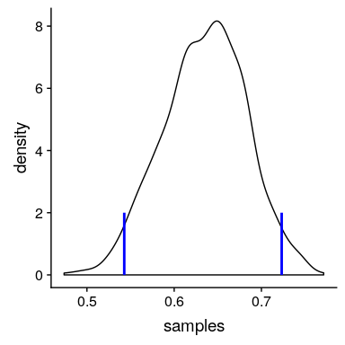圖 11.3 拒絕抽樣示例。黑線表示 P（響應）所有可能值的密度；藍線表示分布的 2.5%和 97.5%，表示 P（響應）估計的 95%可信區間。 這個可信區間的解釋更接近于我們希望從置信區間（但不能）中得到的結果：它告訴我們，95%的概率的值介于這兩個值之間。重要的是，它表明我們對有很高的信心，這意味著該藥物似乎有積極的效果。 ### 11.4.8 不同先驗的影響 在上一個例子中，我們在之前使用了 _ 平面，這意味著我們沒有任何理由相信的任何特定值或多或少是可能的。然而，假設我們是從一些以前的數據開始的：在之前的一項研究中，研究人員測試了 20 個人，發現其中 10 個人的反應是積極的。這將引導我們從先前的信念開始，即治療對 50%的人有效果。我們可以做與上面相同的計算，但是使用我們以前的研究中的信息來通知我們之前的研究（參見圖[11.4](#fig:posteriorDistPrior)）。_ ```r # compute likelihoods for data under all values of p(heads) # using a flat or empirical prior. # here we use the quantized values from .01 to .99 in steps of 0.01 df <- tibble( steps = seq(from = 0.01, to = 0.99, by = 0.01) ) %>% mutate( likelihoods = dbinom(nResponders, 100, steps), priors_flat = dunif(steps) / sum(dunif(steps)), priors_empirical = dbinom(10, 20, steps) / sum(dbinom(10, 20, steps)) ) marginal_likelihood_flat <- sum(dbinom(nResponders, 100, df$steps) * df$priors_flat) marginal_likelihood_empirical <- sum(dbinom(nResponders, 100, df$steps) * df$priors_empirical) df <- df %>% mutate( posteriors_flat = (likelihoods * priors_flat) / marginal_likelihood_flat, posteriors_empirical = (likelihoods * priors_empirical) / marginal_likelihood_empirical ) ```  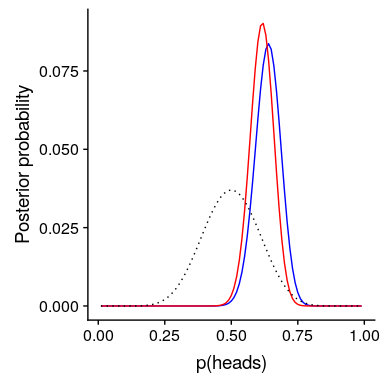圖 11.4 先驗對后驗分布的影響。基于平坦先驗的原始后驗分布用藍色繪制。根據對 20 人中 10 名反應者的觀察，先驗者被畫成黑色虛線，后驗者被畫成紅色。 注意，可能性和邊際可能性并沒有改變——只有先前的改變。手術前改變的效果是將后路拉近新手術前的質量，中心為 0.5。 現在，讓我們看看如果我們以一個更強大的先驗信念來進行分析會發生什么。假設之前的研究沒有觀察到 20 人中有 10 人有反應，而是測試了 500 人，發現 250 人有反應。原則上，這應該給我們一個更強大的先驗，正如我們在圖[11.5](#fig:strongPrior)中所看到的，這就是發生的事情：先驗的集中度要高出 0.5 左右，后驗的集中度也更接近先驗。一般的觀點是貝葉斯推理將先驗信息和似然信息結合起來，并對每一種推理的相對強度進行加權。 ```r # compute likelihoods for data under all values of p(heads) using strong prior. 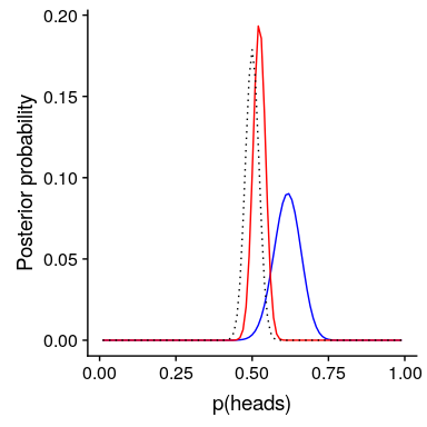df <- df %>% mutate( priors_strong = dbinom(250, 500, steps) / sum(dbinom(250, 500, steps)) ) marginal_likelihood_strong <- sum(dbinom(nResponders, 100, df$steps) * df$priors_strong) df <- df %>% mutate( posteriors_strongprior = (likelihoods * priors_strong) / marginal_likelihood_strong ) ```  圖 11.5：前向強度對后向分布的影響。藍線顯示了 100 人中 50 個人頭使用先驗圖獲得的后驗圖。虛線黑線顯示的是 500 次翻轉中 250 個頭部的先驗圖像，紅線顯示的是基于先驗圖像的后驗圖像。 這個例子也突出了貝葉斯分析的順序性——一個分析的后驗可以成為下一個分析的前驗。 最后，重要的是要認識到，如果先驗足夠強，它們可以完全壓倒數據。假設你有一個絕對先驗，它等于或大于 0.8，這樣你就把所有其他值的先驗概率設置為零。如果我們計算后驗，會發生什么？ ```r # compute likelihoods for data under all values of p(respond) using absolute prior. df <- df %>% mutate( priors_absolute = array(data = 0, dim = length(steps)), priors_absolute = if_else( steps >= 0.8, 1, priors_absolute ), priors_absolute = priors_absolute / sum(priors_absolute) ) marginal_likelihood_absolute <- sum(dbinom(nResponders, 100, df$steps) * df$priors_absolute) df <- df %>% mutate( posteriors_absolute = (likelihoods * priors_absolute) / marginal_likelihood_absolute ) ```  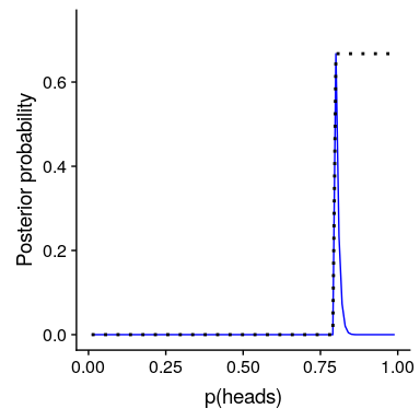圖 11.6：前向強度對后向分布的影響。藍線表示使用絕對先驗得到的后驗值，表示 P（響應）大于等于 0.8。前面的內容顯示在黑色虛線中。 在圖[11.6](#fig:absolutePrior)中，我們發現，在先前設置為零的任何值的后面都存在零密度-數據被絕對先前覆蓋。