# 14 一般線性模型 請記住，在本書的早期，我們描述了統計的基本模型：  其中，我們的一般目標是找到最大限度地減少錯誤的模型，并受一些其他約束（例如保持模型相對簡單，以便我們可以在特定數據集之外進行歸納）。在本章中，我們將重點介紹這種方法的特殊實現，即 _ 一般線性模型 _（或 GLM）。您已經在前面一章中看到了將模型擬合到數據的一般線性模型，我們在 nhanes 數據集中將高度建模為年齡的函數；在這里，我們將更全面地介紹 GLM 的概念及其許多用途。 在討論一般線性模型之前，我們先定義兩個對我們的討論很重要的術語： * _ 因變量 _：這是我們的模型要解釋的結果變量（通常稱為 _y_） * _ 自變量 _：這是一個我們希望用來解釋因變量的變量（通常稱為 _x_）。 可能有多個自變量，但對于本課程，我們的分析中只有一個因變量。 一般線性模型是由獨立變量的 _ 線性組合 _ 組成的，每個獨立變量乘以一個權重（通常稱為希臘字母 beta-），確定相對貢獻。模型預測的自變量。 作為一個例子，讓我們為學習時間和考試成績之間的關系生成一些模擬數據（參見圖[14.1](#fig:StudytimeGrades)）。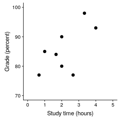 ```r # create simulated data for example set.seed(12345) # the number of points that having a prior class increases grades betas <- c(6, 5) df <- tibble( studyTime = c(2, 3, 5, 6, 6, 8, 10, 12) / 3, priorClass = c(0, 1, 1, 0, 1, 0, 1, 0) ) %>% mutate( grade = studyTime * betas[1] + priorClass * betas[2] + round(rnorm(8, mean = 70, sd = 5)) ) ```  圖 14.1 學習時間與成績的關系 鑒于這些數據，我們可能希望參與三項基本統計活動： * _ 描述一下 _：年級和學習時間之間的關系有多強？ * _ 決定 _：年級和學習時間之間有統計學意義的關系嗎？ * _ 預測 _：給定特定的學習時間，我們期望達到什么級別？ 在最后一章中，我們學習了如何使用相關系數來描述兩個變量之間的關系，因此我們可以使用它來描述這里的關系，并測試相關性是否具有統計意義： ```r # compute correlation between grades and study time corTestResult <- cor.test(df$grade, df$studyTime, alternative = "greater") corTestResult ``` ```r ## ## Pearson's product-moment correlation ## ## data: df$grade and df$studyTime ## t = 2, df = 6, p-value = 0.05 ## alternative hypothesis: true correlation is greater than 0 ## 95 percent confidence interval: ## 0.014 1.000 ## sample estimates: ## cor ## 0.63 ``` 相關性很高，但由于樣本量很小，幾乎沒有達到統計顯著性。