## 14.3 變量之間的相互作用 在前面的模型中，我們假設兩組的學習時間對成績的影響（即回歸斜率）是相同的。但是，在某些情況下，我們可以想象一個變量的效果可能會因另一個變量的值而不同，我們稱之為變量之間的 _ 交互 _。  圖 14.6 咖啡因與公共演講的關系 讓我們用一個新的例子來問這個問題：咖啡因對公眾演講的影響是什么？首先，讓我們生成一些數據并繪制它們。從圖[14.6](#fig:CaffeineSpeaking)來看，似乎沒有關系，我們可以通過對數據進行線性回歸來確認： ```r # perform linear regression with caffeine as independent variable lmResultCaffeine <- lm(speaking ~ caffeine, data = df) summary(lmResultCaffeine) ``` ```r ## ## Call: ## lm(formula = speaking ~ caffeine, data = df) ## ## Residuals: ## Min 1Q Median 3Q Max ## -33.10 -16.02 5.01 16.45 26.98 ## ## Coefficients: ## Estimate Std. Error t value Pr(>|t|) ## (Intercept) -7.413 9.165 -0.81 0.43 ## caffeine 0.168 0.151 1.11 0.28 ## ## Residual standard error: 19 on 18 degrees of freedom ## Multiple R-squared: 0.0642, Adjusted R-squared: 0.0122 ## F-statistic: 1.23 on 1 and 18 DF, p-value: 0.281 ``` 但現在讓我們假設，我們發現研究表明焦慮和非焦慮的人對咖啡因的反應不同。首先，讓我們分別為焦慮和非焦慮的人繪制數據。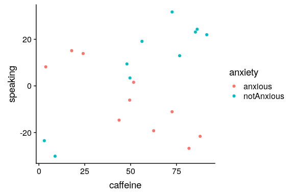  圖 14.7 咖啡因與公共演講的關系，數據點顏色代表焦慮 從圖[14.7](#fig:CaffeineSpeakingAnxiety)可以看出，兩組人的言語和咖啡因之間的關系是不同的，咖啡因改善了無焦慮人群的表現，降低了焦慮人群的表現。我們想創建一個解決這個問題的統計模型。首先，讓我們看看如果在模型中包含焦慮會發生什么。 ```r # compute linear regression adding anxiety to model lmResultCafAnx <- lm(speaking ~ caffeine + anxiety, data = df) summary(lmResultCafAnx) ``` ```r ## ## Call: ## lm(formula = speaking ~ caffeine + anxiety, data = df) ## ## Residuals: ## Min 1Q Median 3Q Max ## -32.97 -9.74 1.35 10.53 25.36 ## ## Coefficients: ## Estimate Std. Error t value Pr(>|t|) ## (Intercept) -12.581 9.197 -1.37 0.19 ## caffeine 0.131 0.145 0.91 0.38 ## anxietynotAnxious 14.233 8.232 1.73 0.10 ## ## Residual standard error: 18 on 17 degrees of freedom ## Multiple R-squared: 0.204, Adjusted R-squared: 0.11 ## F-statistic: 2.18 on 2 and 17 DF, p-value: 0.144 ``` 在這里，我們看到咖啡因和焦慮都沒有明顯的效果，這看起來有點令人困惑。問題是，這一模型試圖符合兩組人對咖啡因說話的同一條線。如果我們想使用單獨的行來擬合它們，我們需要在模型中包含一個 _ 交互 _，這相當于為兩個組中的每個組擬合不同的行；在 r 中，這由符號表示。 ```r # compute linear regression including caffeine X anxiety interaction lmResultInteraction <- lm( speaking ~ caffeine + anxiety + caffeine * anxiety, data = df ) summary(lmResultInteraction) ``` ```r ## ## Call: ## lm(formula = speaking ~ caffeine + anxiety + caffeine * anxiety, ## data = df) ## ## Residuals: ## Min 1Q Median 3Q Max ## -11.385 -7.103 -0.444 6.171 13.458 ## ## Coefficients: ## Estimate Std. Error t value Pr(>|t|) ## (Intercept) 17.4308 5.4301 3.21 0.00546 ** ## caffeine -0.4742 0.0966 -4.91 0.00016 *** ## anxietynotAnxious -43.4487 7.7914 -5.58 4.2e-05 *** ## caffeine:anxietynotAnxious 1.0839 0.1293 8.38 3.0e-07 *** ## --- ## Signif. codes: 0 '***' 0.001 '**' 0.01 '*' 0.05 '.' 0.1 ' ' 1 ## ## Residual standard error: 8.1 on 16 degrees of freedom ## Multiple R-squared: 0.852, Adjusted R-squared: 0.825 ## F-statistic: 30.8 on 3 and 16 DF, p-value: 7.01e-07 ``` 從這些結果中，我們發現咖啡因和焦慮都有顯著的影響（我們稱之為 _ 主要影響 _），以及咖啡因和焦慮之間的相互作用。圖[14.8](#fig:CaffeineAnxietyInteraction)顯示了每組的獨立回歸線。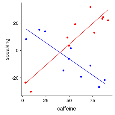  圖 14.8 公眾演講和咖啡因之間的關系，包括與焦慮的互動。這將生成兩條線，分別為每個組建模坡度。 有時我們想比較兩個不同模型的相對擬合，以確定哪個模型更好；我們將其稱為 _ 模型比較 _。對于上面的模型，我們可以使用 r 中的`anova()`命令比較模型的擬合優度（有無交互作用）： ```r anova(lmResultCafAnx, lmResultInteraction) ``` ```r ## Analysis of Variance Table ## ## Model 1: speaking ~ caffeine + anxiety ## Model 2: speaking ~ caffeine + anxiety + caffeine * anxiety ## Res.Df RSS Df Sum of Sq F Pr(>F) ## 1 17 5639 ## 2 16 1046 1 4593 70.3 3e-07 *** ## --- ## Signif. codes: 0 '***' 0.001 '**' 0.01 '*' 0.05 '.' 0.1 ' ' 1 ``` 這告訴我們，有很好的證據表明，比起沒有交互作用的模型，更傾向于有交互作用的模型。在這種情況下，模型比較相對簡單，因為這兩個模型是 _ 嵌套的 _——其中一個模型是另一個模型的簡化版本。與非嵌套模型的模型比較可能會變得更加復雜。