## 13.3 協方差和相關性 量化兩個變量之間關系的一種方法是 _ 協方差 _。記住，單個變量的方差計算如下：  這告訴我們每個觀察值與平均值相差多遠。協方差告訴我們兩個不同的變量在觀測值之間的偏差是否存在關系。定義如下：  當 x 和 y 都高度偏離平均值時，該值將遠離零；如果它們在同一方向上偏離，則協方差為正，而如果它們在相反方向上偏離，則協方差為負。讓我們先看一個玩具的例子。 ```r # create data for toy example of covariance df <- tibble(x = c(3, 5, 8, 10, 12)) %>% mutate(y = x + round(rnorm(n = 5, mean = 0, sd = 2))) %>% mutate( y_dev = y - mean(y), x_dev = x - mean(x) ) %>% mutate(crossproduct = y_dev * x_dev) pander(df) ``` <colgroup><col style="width: 6%"> <col style="width: 6%"> <col style="width: 11%"> <col style="width: 11%"> <col style="width: 19%"></colgroup> | X | 是 | Y 軸偏差 | X 軸偏差 | 叉乘 | | --- | --- | --- | --- | --- | | 三 | 1 個 | -6.6 條 | -4.6 節 | 30.36 天 | | 5 個 | 3 | -4.6 | -第 2.6 條 | 11.96 年 | | 8 個 | 8 | 0.4 倍 | 0.4 | 0.16 分 | | 10 個 | 12 個 | 第 4.4 條 | 第 2.4 條 | 10.56 條 | | 12 | 14 | 第 6.4 條 | 4.4 | 28.16 條 | ```r # compute covariance sprintf("sum of cross products = %.2f", sum(df$crossproduct)) ``` ```r ## [1] "sum of cross products = 81.20" ``` ```r covXY <- sum(df$crossproduct) / (nrow(df) - 1) sprintf("covariance: %.2f", covXY) ``` ```r ## [1] "covariance: 20.30" ``` 我們通常不使用協方差來描述變量之間的關系，因為它隨數據的總體方差水平而變化。相反，我們通常使用 _ 相關系數 _（通常在統計學家 Karl Pearson 之后稱為 _Pearson 相關 _）。通過用兩個變量的標準偏差縮放協方差來計算相關性：  ```r # compute the correlation coefficient corXY <- sum(df$crossproduct) / ((nrow(df) - 1) * sd(df$x) * sd(df$y)) sprintf("correlation coefficient = %.2f", corXY) ``` ```r ## [1] "correlation coefficient = 0.99" ``` 我們還可以使用 r 中的`cor()`函數輕松計算相關值： ```r # compute r using built-in function c <- cor(df$x, df$y) sprintf("correlation coefficient = %.2f", c) ``` ```r ## [1] "correlation coefficient = 0.99" ``` 相關系數是有用的，因為它在-1 和 1 之間變化，不管數據的性質如何-事實上，我們在討論影響大小時已經討論過相關系數。正如我們在上一章關于影響大小的內容中看到的，1 的相關性表示一個完美的線性關系，-1 的相關性表示一個完美的負關系，0 的相關性表示沒有線性關系。 我們可以計算仇恨犯罪數據的相關系數： ```r corGiniHC <- cor( hateCrimes$gini_index, hateCrimes$avg_hatecrimes_per_100k_fbi ) sprintf('correlation coefficient = %.2f',corGiniHC) ``` ```r ## [1] "correlation coefficient = 0.42" ``` ### 13.3.1 相關性假設檢驗 相關值 0.42 似乎表明兩個變量之間的關系相當強，但我們也可以想象，即使沒有關系，這種情況也可能是偶然發生的。我們可以使用一個簡單的公式來測試相關性為零的空假設，該公式允許我們將相關性值轉換為 _t_ 統計：  在零假設下，該統計量以自由度為 t 分布。我們可以使用 r 中的`cor.test()`函數計算： ```r # perform correlation test on hate crime data cor.test( hateCrimes$avg_hatecrimes_per_100k_fbi, hateCrimes$gini_index ) ``` ```r ## ## Pearson's product-moment correlation ## ## data: hateCrimes$avg_hatecrimes_per_100k_fbi and hateCrimes$gini_index ## t = 3, df = 50, p-value = 0.002 ## alternative hypothesis: true correlation is not equal to 0 ## 95 percent confidence interval: ## 0.16 0.63 ## sample estimates: ## cor ## 0.42 ``` 這個測試表明，R 值的可能性很低，這個極限或更高，所以我們將拒絕的無效假設。注意，這個測試假設兩個變量都是正態分布的。 我們也可以通過隨機化來檢驗這一點，在隨機化中，我們重復地改變其中一個變量的值并計算相關性，然后將我們觀察到的相關性值與這個零分布進行比較，以確定我們觀察到的值在零假設下的可能性。結果如圖[13.3](#fig:shuffleCorr)所示。使用隨機化計算的 p 值與 t 檢驗給出的答案相當相似。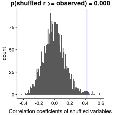 ```r # compute null distribution by shuffling order of variable values # create a function to compute the correlation on the shuffled values shuffleCorr <- function(x, y) { xShuffled <- sample(x) return(cor(xShuffled, y)) } # run this function 2500 times shuffleDist <- replicate( 2500, shuffleCorr(hateCrimes$avg_hatecrimes_per_100k_fbi, hateCrimes$gini_index) ) ```  圖 13.3 零假設下相關值的柱狀圖，通過改變值獲得。觀測值用藍線表示。 ### 13.3.2 穩健相關性 在圖[13.2](#fig:hateCrimeGini)中，您可能注意到了一些有點奇怪的地方——其中一個數據點（哥倫比亞特區的數據點）似乎與其他數據點非常不同。我們稱之為 _ 離群值 _，標準相關系數對離群值非常敏感。例如，在圖[13.4](#fig:outlierCorr)中，我們可以看到一個孤立的數據點是如何導致非常高的正相關值的，即使其他數據點之間的實際關系是完全負的。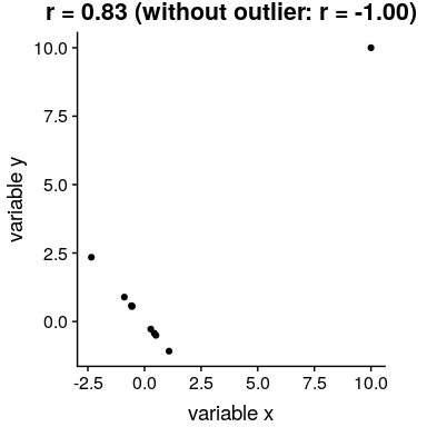  圖 13.4 異常值對相關性影響的模擬示例。如果沒有離群值，其余數據點具有完全的負相關，但單個離群值將相關值更改為高度正相關。 解決離群值問題的一種方法是在排序后，在數據的列組上計算相關性，而不是在數據本身上計算相關性；這被稱為 _ 斯皮爾曼相關性 _。圖[13.4](#fig:outlierCorr)中的 Pearson 相關性為 0.83，而 Spearman 相關性為-0.45，表明等級相關性降低了異常值的影響。 我們可以使用`cor.test`函數計算仇恨犯罪數據的等級相關性： ```r corTestSpearman <- cor.test( hateCrimes$avg_hatecrimes_per_100k_fbi, hateCrimes$gini_index, method = "spearman") corTestSpearman ``` ```r ## ## Spearman's rank correlation rho ## ## data: hateCrimes$avg_hatecrimes_per_100k_fbi and hateCrimes$gini_index ## S = 20000, p-value = 0.8 ## alternative hypothesis: true rho is not equal to 0 ## sample estimates: ## rho ## 0.033 ``` 現在我們看到相關性不再顯著（實際上接近于零），這表明 Fivethirtyeight 博客帖子的聲明可能由于離群值的影響而不正確。 ### 13.3.3 貝葉斯相關分析 我們也可以使用貝葉斯分析來分析五個第八個數據，這有兩個優點。首先，它為我們提供了一個后驗概率——在本例中，相關值超過零的概率。其次，貝葉斯估計將觀察到的證據與 _ 先驗 _ 相結合，從而使相關估計 _ 正則化，有效地將其拉向零。在這里，我們可以使用 bayesmed 包中的`jzs_cor`函數來計算它。_ ```r bayesCor <- jzs_cor( hateCrimes$avg_hatecrimes_per_100k_fbi, hateCrimes$gini_index ) ``` ```r ## Compiling model graph ## Resolving undeclared variables ## Allocating nodes ## Graph information: ## Observed stochastic nodes: 50 ## Unobserved stochastic nodes: 4 ## Total graph size: 230 ## ## Initializing model ``` ```r bayesCor ``` ```r ## $Correlation ## [1] 0.41 ## ## $BayesFactor ## [1] 11 ## ## $PosteriorProbability ## [1] 0.92 ``` 請注意，使用貝葉斯方法估計的相關性略小于使用標準相關系數估計的相關性，這是由于該估計基于證據和先驗的組合，從而有效地將估計縮小到反滲透。但是，請注意，貝葉斯分析對異常值不具有魯棒性，它仍然表示有相當強的證據表明相關性大于零。