## 15.2 t 檢驗作為線性模型 t 檢驗是比較平均值的一種專用工具，但也可以看作是一般線性模型的一種應用。在這種情況下，模型如下所示：  然而，吸煙是一個二元變量，因此我們將其作為一個 _ 虛擬變量 _，正如我們在上一章中討論的那樣，將其設置為吸煙者為 1，不吸煙者為零。在這種情況下，只是兩組之間平均值的差，是編碼為零的組的平均值。我們可以使用`lm()`函數來擬合這個模型，并看到它給出與上面的 t 檢驗相同的 t 統計量： ```r # print summary of linear regression to perform t-test s <- summary(lm(TVHrsNum ~ RegularMarij, data = NHANES_sample)) s ``` ```r ## ## Call: ## lm(formula = TVHrsNum ~ RegularMarij, data = NHANES_sample) ## ## Residuals: ## Min 1Q Median 3Q Max ## -2.810 -1.165 -0.166 0.835 2.834 ## ## Coefficients: ## Estimate Std. Error t value Pr(>|t|) ## (Intercept) 2.165 0.115 18.86 <2e-16 *** ## RegularMarijYes 0.645 0.213 3.02 0.0028 ** ## --- ## Signif. 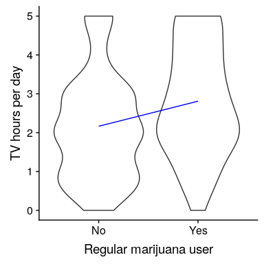codes: 0 '***' 0.001 '**' 0.01 '*' 0.05 '.' 0.1 ' ' 1 ## ## Residual standard error: 1.4 on 198 degrees of freedom ## Multiple R-squared: 0.0441, Adjusted R-squared: 0.0393 ## F-statistic: 9.14 on 1 and 198 DF, p-value: 0.00282 ``` 我們還可以以圖形方式查看 lm（）結果（參見圖[15.2](#fig:ttestFig)）：  圖 15.2 顯示每組數據的小提琴圖，藍色線連接每組的預測值，根據線性模型的結果計算。 在這種情況下，不吸煙者的預測值為（2.17），吸煙者的預測值為（2.81）。 為了計算這個分析的標準誤差，我們可以使用與線性回歸完全相同的方程——因為這實際上只是線性回歸的另一個例子。事實上，如果將上述 t 檢驗中的 p 值與大麻使用變量的線性回歸分析中的 p 值進行比較，您會發現線性回歸分析中的 p 值正好是 t 檢驗中的 p 值的兩倍，因為線性回歸分析正在執行雙尾測試。 ### 15.2.1 比較兩種方法的效果大小 兩種方法之間比較最常用的效果大小是 Cohen's D（如您在第[10](#ci-effect-size-power)章中所記得的），它是用標準誤差單位表示效果的表達式。對于使用上文概述的一般線性模型（即使用單個虛擬編碼變量）估計的 t 檢驗，其表示為：  我們可以從上面的分析輸出中獲得這些值，得出 d=0.47，我們通常將其解釋為中等大小的效果。 我們也可以計算這個分析的，它告訴我們看電視的差異有多大。這個值（在 lm（）分析的摘要中報告）是 0.04，這告訴我們，雖然效果在統計上有顯著意義，但它在電視觀看方面的差異相對較小。