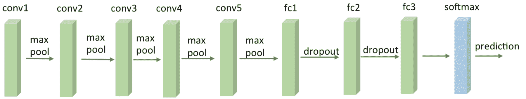
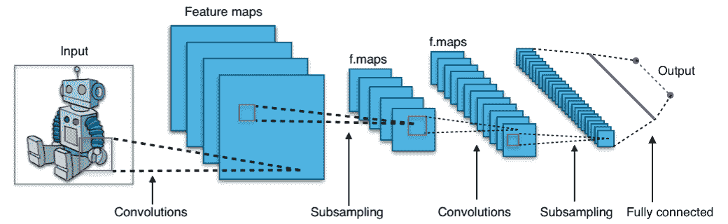
# 四、卷積神經網絡 **卷積神經網絡**（**CNN** 或有時稱為 **ConvNets**）令人著迷。 在短時間內，它們成為一種破壞性技術，打破了從文本，視頻到語音的多個領域中的所有最新技術成果，遠遠超出了最初用于圖像處理的范圍。 在本章中，我們將介紹一些方法，如下所示： * 創建一個卷積網絡對手寫 MNIST 編號進行分類 * 創建一個卷積網絡對 CIFAR-10 進行分類 * 使用 VGG19 遷移風格用于圖像重繪 * 使用預訓練的 VGG16 網絡進行遷移學習 * 創建 DeepDream 網絡 # 介紹 CNN 由許多神經網絡層組成。 卷積和池化兩種不同類型的層通常是交替的。 網絡中每個過濾器的深度從左到右增加。 最后一級通常由一個或多個完全連接的層組成：  [如圖所示，卷積神經網絡的一個示例](https://commons.wikimedia.org/wiki/File:Typical_cnn.png)。 卷積網絡背后有三個主要的直覺：**局部接受域**，**共享權重**和**池化**。 讓我們一起回顧一下。 # 局部接受域 如果我們要保留通常在圖像中發現的空間信息，則使用像素矩陣表示每個圖像會很方便。 然后，編碼局部結構的一種簡單方法是將相鄰輸入神經元的子矩陣連接到屬于下一層的單個隱藏神經元中。 單個隱藏的神經元代表一個局部感受野。 請注意，此操作名為**卷積**，它為這種類型的網絡提供了名稱。 當然，我們可以通過重疊子矩陣來編碼更多信息。 例如，假設每個子矩陣的大小為`5 x 5`，并且這些子矩陣用于`28 x 28`像素的 MNIST 圖像。 然后，我們將能夠在下一個隱藏層中生成`23 x 23`個局部感受野神經元。 實際上，在觸摸圖像的邊界之前，可以僅將子矩陣滑動 23 個位置。 讓我們定義從一層到另一層的特征圖。 當然，我們可以有多個可以從每個隱藏層中獨立學習的特征圖。 例如，我們可以從`28 x 28`個輸入神經元開始處理 MNIST 圖像，然后在下一個隱藏的區域中調用`k`個特征圖，每個特征圖的大小為`23 x 23`神經元（步幅為`5 x 5`）。 # 權重和偏置 假設我們想通過獲得獨立于輸入圖像中放置同一特征的能力來擺脫原始像素表示的困擾。 一個簡單的直覺是對隱藏層中的所有神經元使用相同的權重和偏差集。 這樣，每一層將學習從圖像派生的一組位置無關的潛在特征。 # 一個數學示例 一種了解卷積的簡單方法是考慮應用于矩陣的滑動窗口函數。 在下面的示例中，給定輸入矩陣`I`和內核`K`，我們得到了卷積輸出。 將`3 x 3`內核`K`（有時稱為**過濾器**或**特征檢測器**）與輸入矩陣逐元素相乘，得到輸出卷積矩陣中的一個單元格。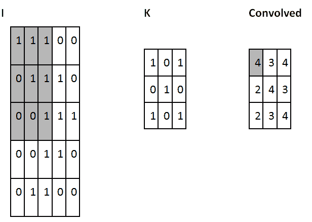 通過在`I`上滑動窗口即可獲得所有其他單元格：  卷積運算的一個示例：用粗體顯示計算中涉及的單元 在此示例中，我們決定在觸摸`I`的邊界后立即停止滑動窗口（因此輸出為`3 x 3`）。 或者，我們可以選擇用零填充輸入（以便輸出為`5 x 5`）。 該決定與所采用的**填充**選擇有關。 另一個選擇是關于**步幅**，這與我們的滑動窗口采用的移位類型有關。 這可以是一個或多個。 較大的跨度將生成較少的內核應用，并且較小的輸出大小，而較小的跨度將生成更多的輸出并保留更多信息。 過濾器的大小，步幅和填充類型是超參數，可以在網絡訓練期間進行微調。 # TensorFlow 中的卷積網絡 在 TensorFlow 中，如果要添加卷積層，我們將編寫以下內容： ```py tf.nn.conv2d(input, filter, strides, padding, use_cudnn_on_gpu=None, data_format=None, name=None) ``` 以下是參數： * `input`：張量必須為以下類型之一：`float32`和`float64`。 * `filter`：張量必須與輸入具有相同的類型。 * `strides`：整數列表。 長度為 1 的 4D。輸入每個維度的滑動窗口的步幅。 必須與格式指定的尺寸順序相同。 * `padding`：來自`SAME`，`VALID`的字符串。 要使用的填充算法的類型。 * `use_cudnn_on_gpu`：可選的布爾值。 默認為`True`。 * `data_format`：來自`NHWC`和`NCHW`的可選字符串。 默認為`NHWC`。 指定輸入和輸出數據的數據格式。 使用默認格式`NHWC`時，數據按以下順序存儲：[`batch`，`in_height`，`in_width`和`in_channels`]。 或者，格式可以是`NCHW`，數據存儲順序為：[`batch`，`in_channels`，`in_height, in_width`]。 * `name`：操作的名稱（可選）。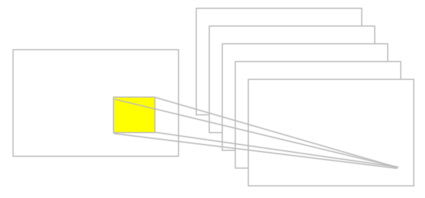 下圖提供了卷積的示例：  卷積運算的一個例子 # 匯聚層 假設我們要總結特征圖的輸出。 同樣，我們可以使用從單個特征圖生成的輸出的空間連續性，并將子矩陣的值聚合為一個單個輸出值，以綜合方式描述與該物理區域相關的含義。 # 最大池 一個簡單而常見的選擇是所謂的**最大池化運算符**，它僅輸出在該區域中觀察到的最大激活。 在 TensorFlow 中，如果要定義大小為`2 x 2`的最大池化層，我們將編寫以下內容： ```py tf.nn.max_pool(value, ksize, strides, padding, data_format='NHWC', name=None) ``` 這些是參數： * `value`：形狀為[`batch`，`height`，`width`，`channels`]且類型為`tf.float32`的 4-D 張量。 * `ksize`：長度`>= 4`的整數的列表。輸入張量每個維度的窗口大小。 * `strides`：長度`>= 4`的整數的列表。輸入張量每個維度的滑動窗口的步幅。 * `padding`：`VALID`或`SAME`的字符串。 * `data_format`：字符串。 支持`NHWC`和`NCHW`。 * `name`：操作的可選名稱。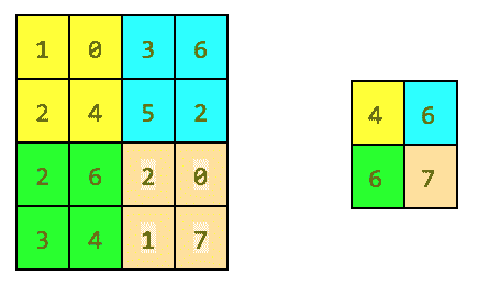 下圖給出了最大池化操作的示例：  池化操作示例 # 平均池化 另一個選擇是“平均池化”，它可以將一個區域簡單地匯總為在該區域中觀察到的激活平均值。 TensorFlow 實現了大量池化層，[可在線獲取完整列表](https://www.tensorflow.org/api_guides/python/nn#Pooling)。簡而言之，所有池化操作僅是對給定區域的匯總操作。 # 卷積網絡摘要 CNN 基本上是卷積的幾層，具有非線性激活函數，并且池化層應用于結果。 每層應用不同的過濾器（數百或數千）。 要理解的主要觀察結果是未預先分配濾波器，而是在訓練階段以最小化合適損失函數的方式來學習濾波器。 已經觀察到，較低的層將學會檢測基本特征，而較高的層將逐漸檢測更復雜的特征，例如形狀或面部。 請注意，得益于合并，后一層中的單個神經元可以看到更多的原始圖像，因此它們能夠組成在前幾層中學習的基本特征。 到目前為止，我們已經描述了 ConvNets 的基本概念。 CNN 在沿時間維度的一維中對音頻和文本數據應用卷積和池化操作，在沿（高度 x 寬度）維的圖像中對二維圖像應用卷積和池化操作，對于沿（高度 x 寬度 x 時間）維的視頻中的三個維度應用卷積和池化操作。 對于圖像，在輸入體積上滑動過濾器會生成一個貼圖，該貼圖為每個空間位置提供過濾器的響應。 換句話說，卷積網絡具有堆疊在一起的多個過濾器，這些過濾器學會了獨立于圖像中的位置來識別特定的視覺特征。 這些視覺特征在網絡的初始層很簡單，然后在網絡的更深層越來越復雜。g操作 # 創建一個卷積網絡對手寫 MNIST 編號進行分類 在本秘籍中，您將學習如何創建一個簡單的三層卷積網絡來預測 MNIST 數字。 深度網絡由具有 ReLU 和最大池化的兩個卷積層以及兩個完全連接的最終層組成。 # 準備 MNIST 是一組 60,000 張代表手寫數字的圖像。 本秘籍的目的是高精度地識別這些數字。 # 操作步驟 讓我們從秘籍開始： 1. 導入`tensorflow`，`matplotlib`，`random`和`numpy`。 然后，導入`minst`數據并執行一鍵編碼。 請注意，TensorFlow 具有一些內置庫來處理`MNIST`，我們將使用它們： ```py from __future__ import division, print_function import tensorflow as tf import matplotlib.pyplot as plt import numpy as np # Import MNIST data from tensorflow.examples.tutorials.mnist import input_data mnist = input_data.read_data_sets("MNIST_data/", one_hot=True) ``` 2. 內省一些數據以了解`MNIST`是什么。 這使我們知道了訓練數據集中有多少張圖像，測試數據集中有多少張圖像。 我們還將可視化一些數字，只是為了理解它們的表示方式。 多單元輸出可以使我們直觀地認識到即使對于人類來說，識別手寫數字也有多困難。 ```py def train_size(num): print ('Total Training Images in Dataset = ' + str(mnist.train.images.shape)) print ('--------------------------------------------------') x_train = mnist.train.images[:num,:] print ('x_train Examples Loaded = ' + str(x_train.shape)) y_train = mnist.train.labels[:num,:] print ('y_train Examples Loaded = ' + str(y_train.shape)) print('') return x_train, y_train def test_size(num): print ('Total Test Examples in Dataset = ' + str(mnist.test.images.shape)) print ('--------------------------------------------------') x_test = mnist.test.images[:num,:] print ('x_test Examples Loaded = ' + str(x_test.shape)) y_test = mnist.test.labels[:num,:] print ('y_test Examples Loaded = ' + str(y_test.shape)) return x_test, y_test def display_digit(num): print(y_train[num]) label = y_train[num].argmax(axis=0) image = x_train[num].reshape([28,28]) plt.title('Example: %d Label: %d' % (num, label)) plt.imshow(image, cmap=plt.get_cmap('gray_r')) plt.show() def display_mult_flat(start, stop): images = x_train[start].reshape([1,784]) for i in range(start+1,stop): images = np.concatenate((images, x_train[i].reshape([1,784]))) plt.imshow(images, cmap=plt.get_cmap('gray_r')) plt.show() x_train, y_train = train_size(55000) display_digit(np.random.randint(0, x_train.shape[0])) display_mult_flat(0,400) ``` 讓我們看一下前面代碼的輸出：   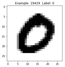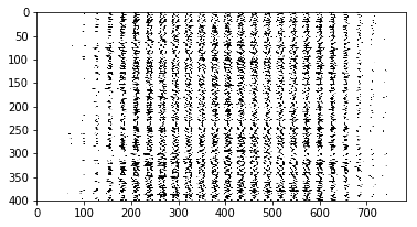MNIST 手寫數字的示例 3. 設置學習參數`batch_size`和`display_step`。 另外，假設 MNIST 圖像共享`28 x 28`像素，請設置`n_input = 784`，表示輸出數字`[0-9]`的輸出`n_classes = 10`，且丟棄概率`= 0.85`： ```py # Parameters learning_rate = 0.001 training_iters = 500 batch_size = 128 display_step = 10 # Network Parameters n_input = 784 # MNIST data input (img shape: 28*28) n_classes = 10 # MNIST total classes (0-9 digits) dropout = 0.85 # Dropout, probability to keep units ``` 4. 設置 TensorFlow 計算圖輸入。 讓我們定義兩個占位符以存儲預測和真實標簽： ```py x = tf.placeholder(tf.float32, [None, n_input]) y = tf.placeholder(tf.float32, [None, n_classes]) keep_prob = tf.placeholder(tf.float32) ``` 5. 使用輸入`x`，權重`W`，偏差`b`和給定的步幅定義卷積層。 激活函數為 ReLU，填充為`SAME`： ```py def conv2d(x, W, b, strides=1): x = tf.nn.conv2d(x, W, strides=[1, strides, strides, 1], padding='SAME') x = tf.nn.bias_add(x, b) return tf.nn.relu(x) ``` 6. 使用輸入`x`，`ksize`和`SAME`填充定義一個最大池化層： ```py def maxpool2d(x, k=2): return tf.nn.max_pool(x, ksize=[1, k, k, 1], strides=[1, k, k, 1], padding='SAME') ``` 7. 用兩個卷積層定義一個卷積網絡，然后是一個完全連接的層，一個退出層和一個最終輸出層： ```py def conv_net(x, weights, biases, dropout): # reshape the input picture x = tf.reshape(x, shape=[-1, 28, 28, 1]) # First convolution layer conv1 = conv2d(x, weights['wc1'], biases['bc1']) # Max Pooling used for downsampling conv1 = maxpool2d(conv1, k=2) # Second convolution layer conv2 = conv2d(conv1, weights['wc2'], biases['bc2']) # Max Pooling used for downsampling conv2 = maxpool2d(conv2, k=2) # Reshape conv2 output to match the input of fully connected layer fc1 = tf.reshape(conv2, [-1, weights['wd1'].get_shape().as_list()[0]]) # Fully connected layer fc1 = tf.add(tf.matmul(fc1, weights['wd1']), biases['bd1']) fc1 = tf.nn.relu(fc1) # Dropout fc1 = tf.nn.dropout(fc1, dropout) # Output the class prediction out = tf.add(tf.matmul(fc1, weights['out']), biases['out']) return out ``` 8. 定義層權重和偏差。 第一轉換層具有`5 x 5`卷積，1 個輸入和 32 個輸出。 第二個卷積層具有`5 x 5`卷積，32 個輸入和 64 個輸出。 全連接層具有`7 x 7 x 64`輸入和 1,024 輸出，而第二層具有 1,024 輸入和 10 輸出，對應于最終數字類別。 所有權重和偏差均使用`randon_normal`分布進行初始化： ```py weights = { # 5x5 conv, 1 input, and 32 outputs 'wc1': tf.Variable(tf.random_normal([5, 5, 1, 32])), # 5x5 conv, 32 inputs, and 64 outputs 'wc2': tf.Variable(tf.random_normal([5, 5, 32, 64])), # fully connected, 7*7*64 inputs, and 1024 outputs 'wd1': tf.Variable(tf.random_normal([7*7*64, 1024])), # 1024 inputs, 10 outputs for class digits 'out': tf.Variable(tf.random_normal([1024, n_classes])) } biases = { 'bc1': tf.Variable(tf.random_normal([32])), 'bc2': tf.Variable(tf.random_normal([64])), 'bd1': tf.Variable(tf.random_normal([1024])), 'out': tf.Variable(tf.random_normal([n_classes])) } ``` 9. 使用給定的權重和偏差構建卷積網絡。 基于`cross_entropy`和`logits`定義`loss`函數，并使用 Adam 優化器來最小化成本。 優化后，計算精度： ```py pred = conv_net(x, weights, biases, keep_prob) cost = tf.reduce_mean(tf.nn.softmax_cross_entropy_with_logits(logits=pred, labels=y)) optimizer = tf.train.AdamOptimizer(learning_rate=learning_rate).minimize(cost) correct_prediction = tf.equal(tf.argmax(pred, 1), tf.argmax(y, 1)) accuracy = tf.reduce_mean(tf.cast(correct_prediction, tf.float32)) init = tf.global_variables_initializer() ``` 10. 啟動圖并迭代`training_iterats`次，每次在輸入中輸入`batch_size`來運行優化器。 請注意，我們使用`mnist.train`數據進行訓練，該數據與`minst`分開。 每個`display_step`都會計算出當前的部分精度。 最后，在 2,048 張測試圖像上計算精度，沒有丟棄。 ```py train_loss = [] train_acc = [] test_acc = [] with tf.Session() as sess: sess.run(init) step = 1 while step <= training_iters: batch_x, batch_y = mnist.train.next_batch(batch_size) sess.run(optimizer, feed_dict={x: batch_x, y: batch_y, keep_prob: dropout}) if step % display_step == 0: loss_train, acc_train = sess.run([cost, accuracy], feed_dict={x: batch_x, y: batch_y, keep_prob: 1.}) print "Iter " + str(step) + ", Minibatch Loss= " + \ "{:.2f}".format(loss_train) + ", Training Accuracy= " + \ "{:.2f}".format(acc_train) # Calculate accuracy for 2048 mnist test images. # Note that in this case no dropout acc_test = sess.run(accuracy, feed_dict={x: mnist.test.images, y: mnist.test.labels, keep_prob: 1.}) print "Testing Accuracy:" + \ "{:.2f}".format(acc_train) train_loss.append(loss_train) train_acc.append(acc_train) test_acc.append(acc_test) step += 1 ``` 11. 繪制每次迭代的 Softmax 損失以及訓練和測試精度： ```py eval_indices = range(0, training_iters, display_step) # Plot loss over time plt.plot(eval_indices, train_loss, 'k-') plt.title('Softmax Loss per iteration') plt.xlabel('Iteration') plt.ylabel('Softmax Loss') plt.show() # Plot train and test accuracy plt.plot(eval_indices, train_acc, 'k-', label='Train Set Accuracy') plt.plot(eval_indices, test_acc, 'r--', label='Test Set Accuracy') plt.title('Train and Test Accuracy') plt.xlabel('Generation') plt.ylabel('Accuracy') plt.legend(loc='lower right') plt.show() ``` 以下是前面代碼的輸出。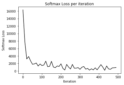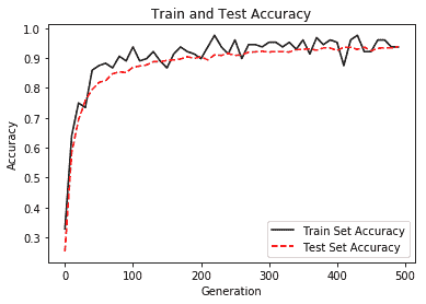 我們首先看一下每次迭代的 Softmax：  損失減少的一個例子 接下來我們看一下訓練和文本的準確率：  訓練和測試準確率提高的示例 # 工作原理 使用卷積網絡，我們將 MNIST 數據集的表現提高了近 95%。 我們的卷積網絡由兩層組成，分別是卷積，ReLU 和最大池化，然后是兩個完全連接的帶有丟棄的層。 訓練以 Adam 為優化器，以 128 的大小批量進行，學習率為 0.001，最大迭代次數為 500。 # 創建一個卷積網絡對 CIFAR-10 進行分類 在本秘籍中，您將學習如何對從 CIFAR-10 拍攝的圖像進行分類。 CIFAR-10 數據集由 10 類 60,000 張`32 x 32`彩色圖像組成，每類 6,000 張圖像。 有 50,000 張訓練圖像和 10,000 張測試圖像。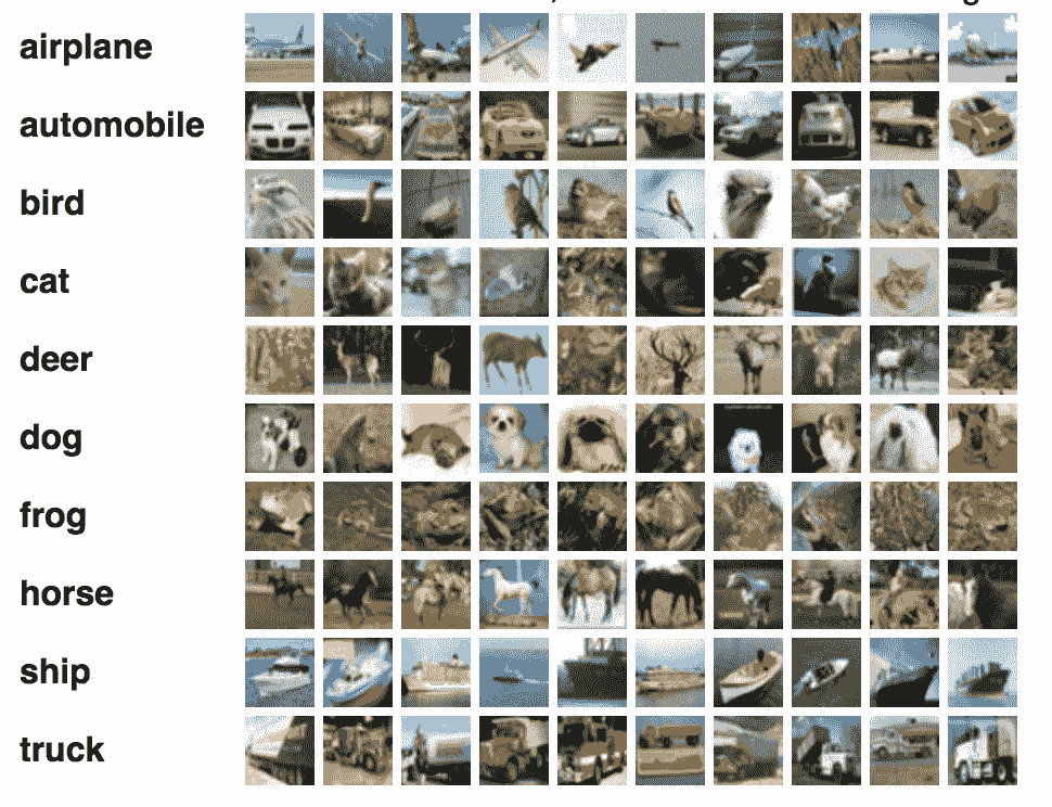 下圖取自[這里](https://www.cs.toronto.edu/~kriz/cifar.html)：  CIFAR 圖像示例 # 準備 在本秘籍中，我們使用`tflearn`-一個更高級別的框架-抽象了一些 TensorFlow 內部結構，使我們可以專注于深度網絡的定義。 TFLearn 可從[這里](http://tflearn.org/)獲得，[該代碼是標準發行版的一部分](https://github.com/tflearn/tflearn/tree/master/examples)。 # 操作步驟 我們按以下步驟進行： 1. 為卷積網絡，`dropout`，`fully_connected`和`max_pool`導入一些`utils`和核心層。 此外，導入一些對圖像處理和圖像增強有用的模塊。 請注意，TFLearn 為卷積網絡提供了一些已經定義的更高層，這使我們可以專注于代碼的定義： ```py from __future__ import division, print_function, absolute_import import tflearn from tflearn.data_utils import shuffle, to_categorical from tflearn.layers.core import input_data, dropout, fully_connected from tflearn.layers.conv import conv_2d, max_pool_2d from tflearn.layers.estimator import regression from tflearn.data_preprocessing import ImagePreprocessing from tflearn.data_augmentation import ImageAugmentation ``` 2. 加載 CIFAR-10 數據，并將其分為`X`列數據，`Y`列標簽，用于測試的`X_test`和用于測試標簽的`Y_test`。 隨機排列`X`和`Y`可能會很有用，以避免取決于特定的數據配置。 最后一步是對`X`和`Y`進行一次熱編碼： ```py # Data loading and preprocessing from tflearn.datasets import cifar10 (X, Y), (X_test, Y_test) = cifar10.load_data() X, Y = shuffle(X, Y) Y = to_categorical(Y, 10) Y_test = to_categorical(Y_test, 10) ``` 3. 將`ImagePreprocessing()`用于零中心（在整個數據集上計算平均值）和 STD 歸一化（在整個數據集上計算 std）。 TFLearn 數據流旨在通過在 GPU 執行模型訓練時在 CPU 上預處理數據來加快訓練速度。 ```py # Real-time data preprocessing img_prep = ImagePreprocessing() img_prep.add_featurewise_zero_center() img_prep.add_featurewise_stdnorm() ``` 4. 通過左右隨機執行以及隨機旋轉來增強數據集。 此步驟是一個簡單的技巧，用于增加可用于訓練的數據： ```py # Real-time data augmentation img_aug = ImageAugmentation() img_aug.add_random_flip_leftright() img_aug.add_random_rotation(max_angle=25.) ``` 5. 使用先前定義的圖像準備和擴充來創建卷積網絡。 網絡由三個卷積層組成。 第一個使用 32 個卷積濾波器，濾波器的大小為 3，激活函數為 ReLU。 之后，有一個`max_pool`層用于縮小尺寸。 然后有兩個級聯的卷積濾波器與 64 個卷積濾波器，濾波器的大小為 3，激活函數為 ReLU。 之后，有一個用于縮小規模的`max_pool`，一個具有 512 個神經元且具有激活函數 ReLU 的全連接網絡，其次是丟棄的可能性為 50%。 最后一層是具有 10 個神經元和激活函數`softmax`的完全連接的網絡，用于確定手寫數字的類別。 請注意，已知這種特定類型的卷積網絡對于 CIFAR-10 非常有效。 在這種特殊情況下，我們將 Adam 優化器與`categorical_crossentropy`和學習率`0.001`結合使用： ```py # Convolutional network building network = input_data(shape=[None, 32, 32, 3], data_preprocessing=img_prep, data_augmentation=img_aug) network = conv_2d(network, 32, 3, activation='relu') network = max_pool_2d(network, 2) network = conv_2d(network, 64, 3, activation='relu') network = conv_2d(network, 64, 3, activation='relu') network = max_pool_2d(network, 2) network = fully_connected(network, 512, activation='relu') network = dropout(network, 0.5) network = fully_connected(network, 10, activation='softmax') network = regression(network, optimizer='adam', loss='categorical_crossentropy', learning_rate=0.001) ``` 6. 實例化卷積網絡并使用`batch_size=96`將訓練運行 50 個周期： ```py # Train using classifier model = tflearn.DNN(network, tensorboard_verbose=0) model.fit(X, Y, n_epoch=50, shuffle=True, validation_set=(X_test, Y_test), show_metric=True, batch_size=96, run_id='cifar10_cnn') ``` # 工作原理 TFLearn 隱藏了 TensorFlow 公開的許多實現細節，并且在許多情況下，它使我們可以專注于具有更高抽象級別的卷積網絡的定義。 我們的管道在 50 次迭代中達到了 88% 的精度。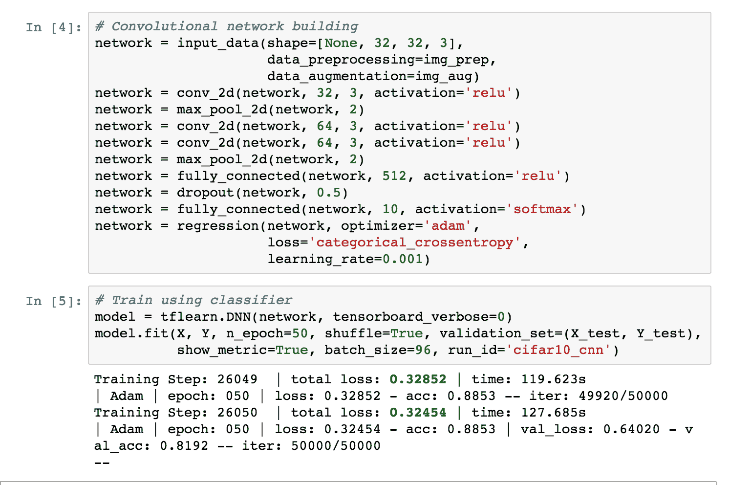 下圖是 Jupyter 筆記本中執行的快照：  Jupyter 執行 CIFAR10 分類的示例 # 更多 要安裝 TFLearn，請參閱[《安裝指南》](http://tflearn.org/installation)，如果您想查看更多示例，可以在線獲取[一長串久經考驗的解決方案](http://tflearn.org/examples/)。 # 使用 VGG19 遷移風格用于圖像重繪 在本秘籍中，您將教計算機如何繪畫。 關鍵思想是擁有繪畫模型圖像，神經網絡可以從該圖像推斷繪畫風格。 然后，此風格將遷移到另一張圖片，并相應地重新粉刷。 該秘籍是對`log0`開發的代碼的修改，[可以在線獲取](https://github.com/log0/neural-style-painting/blob/master/TensorFlow%20Implementation%20of%20A%20Neural%20Algorithm%20of%20Artistic%20Style.ipynb)。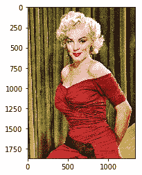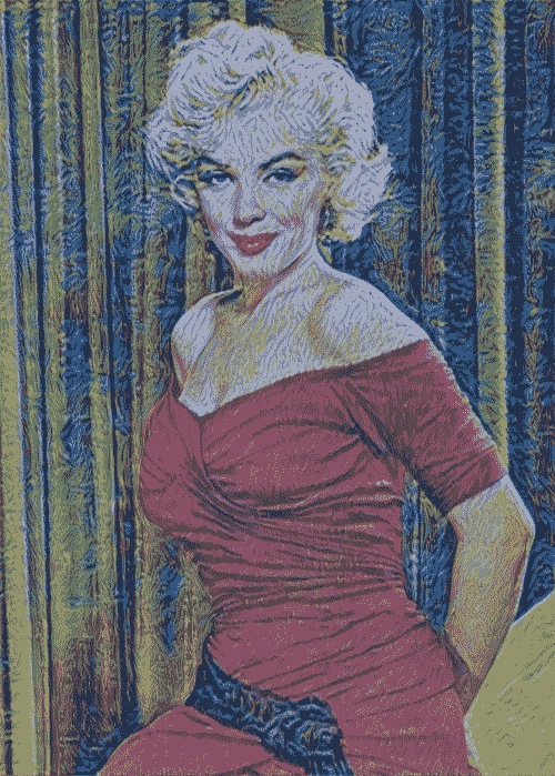 # 準備 我們將實現在論文[《一種藝術風格的神經算法》](https://arxiv.org/abs/1508.06576)中描述的算法，作者是 Leon A. Gatys，亞歷山大 S. Ecker 和 Matthias Bethge。 因此，最好先閱讀[該論文](https://arxiv.org/abs/1508.06576)。 此秘籍將重復使用在線提供的預訓練模型 [VGG19](http://www.vlfeat.org/matconvnet/models/beta16/imagenet-vgg-verydeep-19.mat)，該模型應在本地下載。 我們的風格圖片將是一幅可在線獲得的[梵高著名畫作](https://commons.wikimedia.org/wiki/File:VanGogh-starry_night.jpg)，而我們的內容圖片則是[從維基百科下載的瑪麗蓮夢露的照片](https://commons.wikimedia.org/wiki/File:Marilyn_Monroe_in_1952.jpg)。 內容圖像將根據梵高的風格重新繪制。 # 操作步驟 讓我們從秘籍開始： 1. 導入一些模塊，例如`numpy`，`scipy`，`tensorflow`和`matplotlib`。 然后導入`PIL`來處理圖像。 請注意，由于此代碼在 Jupyter 筆記本上運行，您可以從網上下載該片段，因此添加了片段`%matplotlib inline`： ```py import os import sys import numpy as np import scipy.io import scipy.misc import tensorflow as tf import matplotlib.pyplot as plt from matplotlib.pyplot import imshow from PIL import Image %matplotlib inline from __future__ import division ``` 2. 然后，設置用于學習風格的圖像的輸入路徑，并根據風格設置要重繪的內容圖像的輸入路徑： ```py OUTPUT_DIR = 'output/' # Style image STYLE_IMAGE = 'data/StarryNight.jpg' # Content image to be repainted CONTENT_IMAGE = 'data/Marilyn_Monroe_in_1952.jpg' ``` 3. 然后，我們設置圖像生成過程中使用的噪聲比，以及在重畫內容圖像時要強調的內容損失和風格損失。 除此之外，我們存儲通向預訓練的 VGG 模型的路徑和在 VGG 預訓練期間計算的平均值。 這個平均值是已知的，可以從 VGG 模型的輸入中減去： ```py # how much noise is in the image NOISE_RATIO = 0.6 # How much emphasis on content loss. BETA = 5 # How much emphasis on style loss. ALPHA = 100 # the VGG 19-layer pre-trained model VGG_MODEL = 'data/imagenet-vgg-verydeep-19.mat' # The mean used when the VGG was trained # It is subtracted from the input to the VGG model. 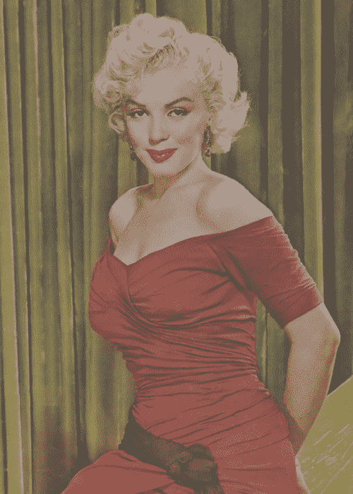MEAN_VALUES = np.array([123.68, 116.779, 103.939]).reshape((1,1,1,3)) ``` 4. 顯示內容圖像只是為了了解它的樣子： ```py content_image = scipy.misc.imread(CONTENT_IMAGE) imshow(content_image) ``` 這是前面代碼的輸出（請注意，此圖像位于[這個頁面](https://commons.wikimedia.org/wiki/File:Marilyn_Monroe_in_1952.jpg)中）：  5. 調整風格圖像的大小并顯示它只是為了了解它的狀態。 請注意，內容圖像和風格圖像現在具有相同的大小和相同數量的顏色通道： ```py style_image = scipy.misc.imread(STYLE_IMAGE) # Get shape of target and make the style image the same target_shape = content_image.shape print "target_shape=", target_shape print "style_shape=", style_image.shape #ratio = target_shape[1] / style_image.shape[1] #print "resize ratio=", ratio style_image = scipy.misc.imresize(style_image, target_shape) scipy.misc.imsave(STYLE_IMAGE, style_image) imshow(style_image) ``` 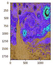這是前面代碼的輸出：  [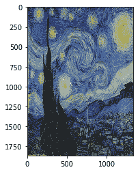文森特·梵高畫作的一個例子](https://commons.wikimedia.org/wiki/File:VanGogh-starry_night_ballance1.jpg) 6. 下一步是按照原始論文中的描述定義 VGG 模型。 請注意，深度學習網絡相當復雜，因為它結合了具有 ReLU 激活函數和最大池的多個卷積網絡層。 另外需要注意的是，在原始論文《風格遷移》（Leon A. Gatys，Alexander S. Ecker 和 Matthias Bethge 撰寫的《一種藝術風格的神經算法》）中，許多實驗表明，平均合并實際上優于最大池化。 因此，我們將改用平均池： ```py def load_vgg_model(path, image_height, image_width, color_channels): """ Returns the VGG model as defined in the paper 0 is conv1_1 (3, 3, 3, 64) 1 is relu 2 is conv1_2 (3, 3, 64, 64) 3 is relu 4 is maxpool 5 is conv2_1 (3, 3, 64, 128) 6 is relu 7 is conv2_2 (3, 3, 128, 128) 8 is relu 9 is maxpool 10 is conv3_1 (3, 3, 128, 256) 11 is relu 12 is conv3_2 (3, 3, 256, 256) 13 is relu 14 is conv3_3 (3, 3, 256, 256) 15 is relu 16 is conv3_4 (3, 3, 256, 256) 17 is relu 18 is maxpool 19 is conv4_1 (3, 3, 256, 512) 20 is relu 21 is conv4_2 (3, 3, 512, 512) 22 is relu 23 is conv4_3 (3, 3, 512, 512) 24 is relu 25 is conv4_4 (3, 3, 512, 512) 26 is relu 27 is maxpool 28 is conv5_1 (3, 3, 512, 512) 29 is relu 30 is conv5_2 (3, 3, 512, 512) 31 is relu 32 is conv5_3 (3, 3, 512, 512) 33 is relu 34 is conv5_4 (3, 3, 512, 512) 35 is relu 36 is maxpool 37 is fullyconnected (7, 7, 512, 4096) 38 is relu 39 is fullyconnected (1, 1, 4096, 4096) 40 is relu 41 is fullyconnected (1, 1, 4096, 1000) 42 is softmax """ vgg = scipy.io.loadmat(path) vgg_layers = vgg['layers'] def _weights(layer, expected_layer_name): """ Return the weights and bias from the VGG model for a given layer. """ W = vgg_layers[0][layer][0][0][0][0][0] b = vgg_layers[0][layer][0][0][0][0][1] layer_name = vgg_layers[0][layer][0][0][-2] assert layer_name == expected_layer_name return W, b def _relu(conv2d_layer): """ Return the RELU function wrapped over a TensorFlow layer. Expects a Conv2d layer input. """ return tf.nn.relu(conv2d_layer) def _conv2d(prev_layer, layer, layer_name): """ Return the Conv2D layer using the weights, biases from the VGG model at 'layer'. """ W, b = _weights(layer, layer_name) W = tf.constant(W) b = tf.constant(np.reshape(b, (b.size))) return tf.nn.conv2d( prev_layer, filter=W, strides=[1, 1, 1, 1], padding='SAME') + b def _conv2d_relu(prev_layer, layer, layer_name): """ Return the Conv2D + RELU layer using the weights, biases from the VGG model at 'layer'. """ return _relu(_conv2d(prev_layer, layer, layer_name)) def _avgpool(prev_layer): """ Return the AveragePooling layer. """ return tf.nn.avg_pool(prev_layer, ksize=[1, 2, 2, 1], strides=[1, 2, 2, 1], padding='SAME') # Constructs the graph model. graph = {} graph['input'] = tf.Variable(np.zeros((1, image_height, image_width, color_channels)), dtype = 'float32') graph['conv1_1'] = _conv2d_relu(graph['input'], 0, 'conv1_1') graph['conv1_2'] = _conv2d_relu(graph['conv1_1'], 2, 'conv1_2') graph['avgpool1'] = _avgpool(graph['conv1_2']) graph['conv2_1'] = _conv2d_relu(graph['avgpool1'], 5, 'conv2_1') graph['conv2_2'] = _conv2d_relu(graph['conv2_1'], 7, 'conv2_2') graph['avgpool2'] = _avgpool(graph['conv2_2']) graph['conv3_1'] = _conv2d_relu(graph['avgpool2'], 10, 'conv3_1') graph['conv3_2'] = _conv2d_relu(graph['conv3_1'], 12, 'conv3_2') graph['conv3_3'] = _conv2d_relu(graph['conv3_2'], 14, 'conv3_3') graph['conv3_4'] = _conv2d_relu(graph['conv3_3'], 16, 'conv3_4') graph['avgpool3'] = _avgpool(graph['conv3_4']) graph['conv4_1'] = _conv2d_relu(graph['avgpool3'], 19, 'conv4_1') graph['conv4_2'] = _conv2d_relu(graph['conv4_1'], 21, 'conv4_2') graph['conv4_3'] = _conv2d_relu(graph['conv4_2'], 23, 'conv4_3') graph['conv4_4'] = _conv2d_relu(graph['conv4_3'], 25, 'conv4_4') graph['avgpool4'] = _avgpool(graph['conv4_4']) graph['conv5_1'] = _conv2d_relu(graph['avgpool4'], 28, 'conv5_1') graph['conv5_2'] = _conv2d_relu(graph['conv5_1'], 30, 'conv5_2') graph['conv5_3'] = _conv2d_relu(graph['conv5_2'], 32, 'conv5_3') graph['conv5_4'] = _conv2d_relu(graph['conv5_3'], 34, 'conv5_4') graph['avgpool5'] = _avgpool(graph['conv5_4']) return graph ``` 7. 定義內容`loss`函數，如原始論文中所述： ```py def content_loss_func(sess, model): """ Content loss function as defined in the paper. """ def _content_loss(p, x): # N is the number of filters (at layer l). N = p.shape[3] # M is the height times the width of the feature map (at layer l). M = p.shape[1] * p.shape[2] return (1 / (4 * N * M)) * tf.reduce_sum(tf.pow(x - p, 2)) return _content_loss(sess.run(model['conv4_2']), model['conv4_2']) ``` 8. 定義我們要重用的 VGG 層。 如果我們希望具有更柔和的特征，則需要增加較高層的權重（`conv5_1`）和降低較低層的權重（`conv1_1`）。 如果我們想擁有更難的特征，我們需要做相反的事情： ```py STYLE_LAYERS = [ ('conv1_1', 0.5), ('conv2_1', 1.0), ('conv3_1', 1.5), ('conv4_1', 3.0), ('conv5_1', 4.0), ] ``` 9. 定義風格損失函數，如原始論文中所述： ```py def style_loss_func(sess, model): """ Style loss function as defined in the paper. """ def _gram_matrix(F, N, M): """ The gram matrix G. """ Ft = tf.reshape(F, (M, N)) return tf.matmul(tf.transpose(Ft), Ft) def _style_loss(a, x): """ The style loss calculation. """ # N is the number of filters (at layer l). N = a.shape[3] # M is the height times the width of the feature map (at layer l). M = a.shape[1] * a.shape[2] # A is the style representation of the original image (at layer l). A = _gram_matrix(a, N, M) # G is the style representation of the generated image (at layer l). G = _gram_matrix(x, N, M) result = (1 / (4 * N**2 * M**2)) * tf.reduce_sum(tf.pow(G - A, 2)) return result E = [_style_loss(sess.run(model[layer_name]), model[layer_name]) for layer_name, _ in STYLE_LAYERS] W = [w for _, w in STYLE_LAYERS] loss = sum([W[l] * E[l] for l in range(len(STYLE_LAYERS))]) return loss ``` 10. 定義一個函數以生成噪聲圖像，并將其與內容圖像按給定比例混合。 定義兩種輔助方法來預處理和保存圖像： ```py def generate_noise_image(content_image, noise_ratio = NOISE_RATIO): """ Returns a noise image intermixed with the content image at a certain ratio. """ noise_image = np.random.uniform( -20, 20, (1, content_image[0].shape[0], content_image[0].shape[1], content_image[0].shape[2])).astype('float32') # White noise image from the content representation. Take a weighted average # of the values input_image = noise_image * noise_ratio + content_image * (1 - noise_ratio) return input_image def process_image(image): # Resize the image for convnet input, there is no change but just # add an extra dimension. image = np.reshape(image, ((1,) + image.shape)) # Input to the VGG model expects the mean to be subtracted. image = image - MEAN_VALUES return image def save_image(path, image): # Output should add back the mean. image = image + MEAN_VALUES # Get rid of the first useless dimension, what remains is the image. image = image[0] image = np.clip(image, 0, 255).astype('uint8') scipy.misc.imsave(path, image) ``` 11. 開始一個 TensorFlow 交互式會話： ```py sess = tf.InteractiveSession() ``` 12. 加載處理后的內容圖像并顯示： ```py content_image = load_image(CONTENT_IMAGE) imshow(content_image[0]) ``` 我們得到以下代碼的輸出（請注意，我們使用了來自[這里](https://commons.wikimedia.org/wiki/File:Marilyn_Monroe_in_1952.jpg)的圖像）：  13. 加載處理后的風格圖像并顯示它： ```py style_image = load_image(STYLE_IMAGE) imshow(style_image[0]) ``` 內容如下：  14. 加載`model`并顯示： ```py model = load_vgg_model(VGG_MODEL, style_image[0].shape[0], style_image[0].shape[1], style_image[0].shape[2]) print(model) ``` 15. 生成用于啟動重新繪制的隨機噪聲圖像： ```py input_image = generate_noise_image(content_image) imshow(input_image[0]) ``` 16. 運行 TensorFlow 會話： ```py sess.run(tf.initialize_all_variables()) ``` 17. 用相應的圖像構造`content_loss`和`sytle_loss`： ```py # Construct content_loss using content_image. sess.run(model['input'].assign(content_image)) content_loss = content_loss_func(sess, model) # Construct style_loss using style_image. sess.run(model['input'].assign(style_image)) style_loss = style_loss_func(sess, model) ``` 18. 將`total_loss`構造為`content_loss`和`sytle_loss`的加權組合： ```py # Construct total_loss as weighted combination of content_loss and sytle_loss total_loss = BETA * content_loss + ALPHA * style_loss ``` 19. 建立一個優化器以最大程度地減少總損失。 在這種情況下，我們采用 Adam 優化器： ```py # The content is built from one layer, while the style is from five # layers. Then we minimize the total_loss optimizer = tf.train.AdamOptimizer(2.0) train_step = optimizer.minimize(total_loss) ``` 20. 使用輸入圖像啟動網絡： ```py sess.run(tf.initialize_all_variables()) sess.run(model['input'].assign(input_image)) ``` 21. 對模型運行固定的迭代次數，并生成中間的重繪圖像： ```py sess.run(tf.initialize_all_variables()) sess.run(model['input'].assign(input_image)) print "started iteration" for it in range(ITERATIONS): sess.run(train_step) print it , " " if it%100 == 0: # Print every 100 iteration. 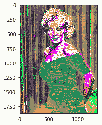mixed_image = sess.run(model['input']) print('Iteration %d' % (it)) print('sum : ', sess.run(tf.reduce_sum(mixed_image))) print('cost: ', sess.run(total_loss)) if not os.path.exists(OUTPUT_DIR): os.mkdir(OUTPUT_DIR) filename = 'output/%d.png' % (it) save_image(filename, mixed_image) ``` 22. 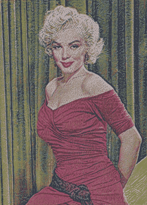在此圖像中，我們顯示了在 200、400 和 600 次迭代后如何重新繪制內容圖像：    風格遷移的例子 # 工作原理 在本秘籍中，我們已經看到了如何使用風格轉換來重繪內容圖像。 風格圖像已作為神經網絡的輸入提供，該網絡學習了定義畫家采用的風格的關鍵方面。 這些方面已用于將風格遷移到內容圖像。 # 更多 自 2015 年提出原始建議以來，風格轉換一直是活躍的研究領域。已經提出了許多新想法來加速計算并將風格轉換擴展到視頻分析。 其中有兩個結果值得一提 這篇文章是 [Logan Engstrom](https://github.com/lengstrom/fast-style-transfer/) 的快速風格轉換，介紹了一種非常快速的實現，該實現也可以與視頻一起使用。 通過 [deepart](https://deepart.io/) 網站，您可以播放自己的圖像，并以自己喜歡的藝術家的風格重新繪制圖片。 還提供了 Android 應用，iPhone 應用和 Web 應用。 # 將預訓練的 VGG16 網絡用于遷移學習 在本秘籍中，我們將討論遷移學習，這是一種非常強大的深度學習技術，在不同領域中都有許多應用。 直覺非常簡單，可以用類推來解釋。 假設您想學習一種新的語言，例如西班牙語，那么從另一種語言（例如英語）已經知道的內容開始可能會很有用。 按照這種思路，計算機視覺研究人員現在通常使用經過預訓練的 CNN 來生成新穎任務的表示形式，其中數據集可能不足以從頭訓練整個 CNN。 另一個常見的策略是采用經過預先訓練的 ImageNet 網絡，然后將整個網絡微調到新穎的任務。 此處提出的示例的靈感來自 [Francois Chollet 在 Keras 的著名博客文章](https://blog.keras.io/building-powerful-image-classification-models-using-very-little-data.html)。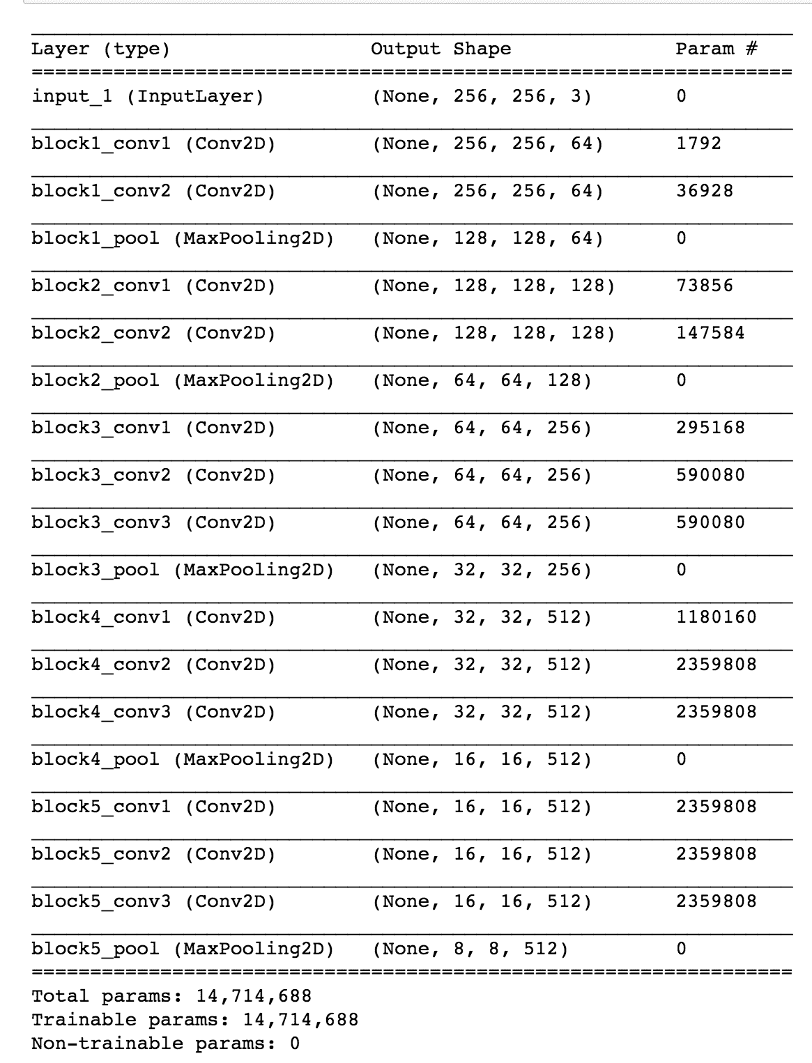 # 準備 想法是使用在大型數據集（如 ImageNet）上預訓練的 VGG16 網絡。 請注意，訓練在計算上可能會相當昂貴，因此可以重用已經預先訓練的網絡：  A VGG16 Network 那么，如何使用 VGG16？ Keras 使該庫變得容易，因為該庫具有可作為庫使用的標準 VGG16 應用，并且自動下載了預先計算的權重。 請注意，我們明確省略了最后一層，并用我們的自定義層替換了它，這將在預構建的 VGG16 的頂部進行微調。 在此示例中，您將學習如何對 Kaggle 提供的貓狗圖像進行分類。 # 操作步驟 我們按以下步驟進行： 1. 從 Kaggle（https://www.kaggle.com/c/dogs-vs-cats/data）下載貓狗數據，并創建一個包含兩個子目錄的數據目錄，`train`和`validation`，每個子目錄都有兩個附加子目錄， 狗和貓。 2. 導入 Keras 模塊，這些模塊將在以后的計算中使用，并保存一些有用的常量： ```py from keras import applications from keras.preprocessing.image import ImageDataGenerator from keras import optimizers from keras.models import Sequential, Model from keras.layers import Dropout, Flatten, Dense from keras import optimizers img_width, img_height = 256, 256 batch_size = 16 epochs = 50 train_data_dir = 'data/dogs_and_cats/train' validation_data_dir = 'data/dogs_and_cats/validation' #OUT CATEGORIES OUT_CATEGORIES=1 #number of train, validation samples nb_train_samples = 2000 nb_validation_samples = ``` 3. 將預訓練的圖像加載到 ImageNet VGG16 網絡上，并省略最后一層，因為我們將在預構建的 VGG16 的頂部添加自定義分類網絡并替換最后的分類層： ```py # load the VGG16 model pretrained on imagenet base_model = applications.VGG16(weights = "imagenet", include_top=False, input_shape = (img_width, img_height, 3)) base_model.summary() ``` 這是前面代碼的輸出：  4. 凍結一定數量的較低層用于預訓練的 VGG16 網絡。 在這種情況下，我們決定凍結最初的 15 層： ```py # Freeze the 15 lower layers for layer in base_model.layers[:15]: layer.trainable = False ``` 5. 添加一組自定義的頂層用于分類： ```py # Add custom to layers # build a classifier model to put on top of the convolutional model top_model = Sequential() top_model.add(Flatten(input_shape=base_model.output_shape[1:])) top_model.add(Dense(256, activation='relu')) top_model.add(Dropout(0.5)) top_model.add(Dense(OUT_CATEGORIES, activation='sigmoid')) ``` 6. 定制網絡應單獨進行預訓練，在這里，為簡單起見，我們省略了這一部分，將這一任務留給了讀者： ```py #top_model.load_weights(top_model_weights_path) ``` 7. 創建一個新網絡，該網絡與預訓練的 VGG16 網絡和我們的預訓練的自定義網絡并置： ```py # creating the final model, a composition of # pre-trained and model = Model(inputs=base_model.input, outputs=top_model(base_model.output)) # compile the model model.compile(loss = "binary_crossentropy", optimizer = optimizers.SGD(lr=0.0001, momentum=0.9), metrics=["accuracy"]) ``` 8. 重新訓練并列的新模型，仍將 VGG16 的最低 15 層凍結。 在這個特定的例子中，我們還使用圖像增幅器來增加訓練集： ```py # Initiate the train and test generators with data Augumentation train_datagen = ImageDataGenerator( rescale = 1./255, horizontal_flip = True) test_datagen = ImageDataGenerator(rescale=1\. / 255) train_generator = train_datagen.flow_from_directory( train_data_dir, target_size=(img_height, img_width), batch_size=batch_size, class_mode='binary') validation_generator = test_datagen.flow_from_directory( validation_data_dir, target_size=(img_height, img_width), batch_size=batch_size, class_mode='binary', shuffle=False) model.fit_generator( train_generator, steps_per_epoch=nb_train_samples // batch_size, epochs=epochs, validation_data=validation_generator, validation_steps=nb_validation_samples // batch_size, verbose=2, workers=12) ``` 9. 在并置的網絡上評估結果： ```py score = model.evaluate_generator(validation_generator, nb_validation_samples/batch_size) scores = model.predict_generator(validation_generator, nb_validation_samples/batch_size) ``` # 工作原理 標準的 VGG16 網絡已經在整個 ImageNet 上進行了預訓練，并具有從互聯網下載的預先計算的權重。 然后，將該網絡與也已單獨訓練的自定義網絡并置。 然后，并列的網絡作為一個整體進行了重新訓練，使 VGG16 的 15 個較低層保持凍結。 這種組合非常有效。 通過對網絡在 ImageNet 上學到的知識進行遷移學習，將其應用于我們的新特定領域，從而執行微調分類任務，它可以節省大量的計算能力，并重復使用已為 VGG16 執行的工作。 # 更多 根據特定的分類任務，需要考慮一些經驗法則： * 如果新數據集很小并且類似于 ImageNet 數據集，那么我們可以凍結所有 VGG16 網絡并僅重新訓練自定義網絡。 通過這種方式，我們還將并置網絡的過擬合風險降至最低： ＃凍結`base_model.layers`中所有較低的層：`layer.trainable = False` * 如果新數據集很大且類似于 ImageNet 數據集，則我們可以重新訓練整個并列的網絡。 我們仍然將預先計算的權重作為起點，并進行一些迭代以進行微調： ＃取消凍結`model.layers`中所有較低層的層：`layer.trainable = True` * 如果新數據集與 ImageNet 數據集非常不同，則在實踐中，使用預訓練模型中的權重進行初始化可能仍然很好。 在這種情況下，我們將有足夠的數據和信心來調整整個網絡。 可以在[這里](http://cs231n.github.io/transfer-learning/)在線找到更多信息。 # 創建 DeepDream 網絡 Google 于 2014 年訓練了神經網絡以應對 **ImageNet 大規模視覺識別挑戰**（**ILSVRC**），并于 2015 年 7 月將其開源。[“深入了解卷積”](https://arxiv.org/abs/1409.4842)中介紹了原始算法。 網絡學會了每個圖像的表示。 較低的層學習諸如線條和邊緣之類的底層特征，而較高的層則學習諸如眼睛，鼻子，嘴等更復雜的圖案。 因此，如果嘗試在網絡中代表更高的級別，我們將看到從原始 ImageNet 提取的各種不同特征的混合，例如鳥的眼睛和狗的嘴巴。 考慮到這一點，如果我們拍攝一張新圖像并嘗試使與網絡上層的相似性最大化，那么結果就是一張新的有遠見的圖像。 在這個有遠見的圖像中，較高層學習的某些模式在原始圖像中被夢到（例如，想象中）。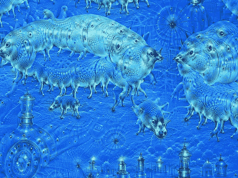 這是此類有遠見的圖像的示例：  [如以下所示的 Google DeepDreams 示例](https://commons.wikimedia.org/wiki/File:Aurelia-aurita-3-0009.jpg) # 準備 從網上下載預訓練的 [Inception 模型](https://github.com/martinwicke/tensorflow-tutorial/blob/master/tensorflow_inception_graph.pb)。 # 操作步驟 我們按以下步驟進行操作： 1. 導入`numpy`進行數值計算，導入`functools`定義已填充一個或多個參數的部分函數，??導入 Pillow 進行圖像處理，并導入`matplotlib`呈現圖像： ```py import numpy as np from functools import partial import PIL.Image import tensorflow as tf import matplotlib.pyplot as plt ``` 2. 設置內容圖像和預訓練模型的路徑。 從只是隨機噪聲的種子圖像開始： ```py content_image = 'data/gulli.jpg' # start with a gray image with a little noise img_noise = np.random.uniform(size=(224,224,3)) + 100.0 model_fn = 'data/tensorflow_inception_graph.pb' ``` 3. 在圖表中加載從互聯網下載的 Inception 網絡。 初始化 TensorFlow 會話，使用`FastGFile(..)`加載圖，然后使用`ParseFromstring(..)`解析圖。 之后，使用`placeholder(..)`方法創建一個輸入作為占位符。 `imagenet_mean`是一個預先計算的常數，將從我們的內容圖像中刪除以標準化數據。 實際上，這是在訓練過程中觀察到的平均值，歸一化可以更快地收斂。 該值將從輸入中減去，并存儲在`t_preprocessed`變量中，該變量然后用于加載圖定義： ```py # load the graph graph = tf.Graph() sess = tf.InteractiveSession(graph=graph) with tf.gfile.FastGFile(model_fn, 'rb') as f: graph_def = tf.GraphDef() graph_def.ParseFromString(f.read()) t_input = tf.placeholder(np.float32, name='input') # define the input tensor imagenet_mean = 117.0 t_preprocessed = tf.expand_dims(t_input-imagenet_mean, 0) tf.import_graph_def(graph_def, {'input':t_preprocessed}) ``` 4. 定義一些`util`函數以可視化圖像并將 TF-graph 生成函數轉換為常規 Python 函數（請參見以下示例以調整大小）： ```py # helper #pylint: disable=unused-variable def showarray(a): a = np.uint8(np.clip(a, 0, 1)*255) plt.imshow(a) plt.show() def visstd(a, s=0.1): '''Normalize the image range for visualization''' return (a-a.mean())/max(a.std(), 1e-4)*s + 0.5 def T(layer): '''Helper for getting layer output tensor''' return graph.get_tensor_by_name("import/%s:0"%layer) def tffunc(*argtypes): '''Helper that transforms TF-graph generating function into a regular one. See "resize" function below. ''' placeholders = list(map(tf.placeholder, argtypes)) def wrap(f): out = f(*placeholders) def wrapper(*args, **kw): return out.eval(dict(zip(placeholders, args)), session=kw.get('session')) return wrapper return wrap def resize(img, size): img = tf.expand_dims(img, 0) return tf.image.resize_bilinear(img, size)[0,:,:,:] resize = tffunc(np.float32, np.int32)(resize) ``` 5. 計算圖像上的梯度上升。 為了提高效率，請應用分塊計算，其中在不同分塊上計算單獨的梯度上升。 將隨機移位應用于圖像，以在多次迭代中模糊圖塊邊界： ```py def calc_grad_tiled(img, t_grad, tile_size=512): '''Compute the value of tensor t_grad over the image in a tiled way. Random shifts are applied to the image to blur tile boundaries over multiple iterations.''' sz = tile_size h, w = img.shape[:2] sx, sy = np.random.randint(sz, size=2) img_shift = np.roll(np.roll(img, sx, 1), sy, 0) grad = np.zeros_like(img) for y in range(0, max(h-sz//2, sz),sz): for x in range(0, max(w-sz//2, sz),sz): sub = img_shift[y:y+sz,x:x+sz] g = sess.run(t_grad, {t_input:sub}) grad[y:y+sz,x:x+sz] = g return np.roll(np.roll(grad, -sx, 1), -sy, 0) ``` 6. 定義優化對象以減少輸入層的均值。 `gradient`函數允許我們通過考慮輸入張量來計算優化張量的符號梯度。 為了提高效率，將圖像分成多個八度，然后調整大小并添加到八度數組中。 然后，對于每個八度，我們使用`calc_grad_tiled`函數： ```py def render_deepdream(t_obj, img0=img_noise, iter_n=10, step=1.5, octave_n=4, octave_scale=1.4): t_score = tf.reduce_mean(t_obj) # defining the optimization objective t_grad = tf.gradients(t_score, t_input)[0] # behold the power of automatic differentiation! # split the image into a number of octaves img = img0 octaves = [] for _ in range(octave_n-1): hw = img.shape[:2] lo = resize(img, np.int32(np.float32(hw)/octave_scale)) hi = img-resize(lo, hw) img = lo octaves.append(hi) # generate details octave by octave for octave in range(octave_n): if octave>0: hi = octaves[-octave] img = resize(img, hi.shape[:2])+hi for _ in range(iter_n): g = calc_grad_tiled(img, t_grad) img += g*(step / (np.abs(g).mean()+1e-7)) #this will usually be like 3 or 4 octaves #Step 5 output deep dream image via matplotlib showarray(img/255.0) ``` 7. 加載特定的內容圖像并開始做夢。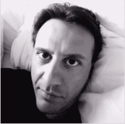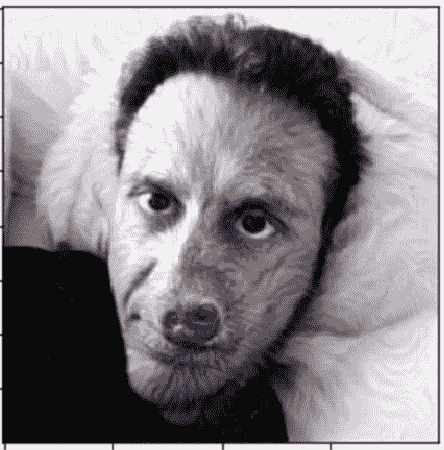 在此示例中，作者的面孔已轉變為類似于狼的事物：   DeepDream 轉換的示例。 其中一位作家變成了狼 # 工作原理 神經網絡存儲訓練圖像的抽象：較低的層存儲諸如線條和邊緣之類的特征，而較高的層則存儲諸如眼睛，面部和鼻子之類的更復雜的圖像特征。 通過應用梯度上升過程，我們最大化了`loss`函數，并有助于發現類似于高層存儲的圖案的內容圖像。 這導致了網絡看到虛幻圖像的夢想。 # 更多 許多網站都允許您直接玩 DeepDream。 我特別喜歡[`DeepArt.io`](https://deepart.io/)，它允許您上傳內容圖像和風格圖像并在云上進行學習。 # 另見 在 2015 年發布初步結果之后，還發布了許多有關 DeepDream 的新論文和博客文章： ```py DeepDream: A code example to visualize Neural Networks--https://research.googleblog.com/2015/07/deepdream-code-example-for-visualizing.html When Robots Hallucinate, LaFrance, Adrienne--https://www.theatlantic.com/technology/archive/2015/09/robots-hallucinate-dream/403498/ ``` 此外，了解如何可視化預訓練網絡的每一層并更好地了解網絡如何記憶較低層的基本特征以及較高層的較復雜特征可能會很有趣。 在線提供有關此主題的有趣博客文章： * [卷積神經網絡如何看待世界](https://blog.keras.io/category/demo.html)