# 六、使用 TensorFlow 2 識別圖像 本章分為兩部分，但我們將同時學習使用 TensorFlow 進行圖像分類。 在本章中，我們將涵蓋以下主要主題： * QuickDraw – 使用 TensorFlow 進行圖像分類 * 使用 TensorFlow 的 CIFAR 10 圖像分類 在第一部分中，我們將使用在前幾章中學到的技術開發 TensorFlow 2 模型以進行圖像識別，尤其是第 2 章， “Keras，TensorFlow 2 的高級 API”。 這將使我們能夠看到如何使用 TensorFlow 2 將所有相關技術結合在一起來創建，訓練和評估完整的模型。我們將利用 Google 提供的 QuickDraw 圖片數據集可幫助您解決此問題。 # QuickDraw – 使用 TensorFlow 進行圖像分類 我們將使用從 Google QuickDraw 拍攝的圖像數據集。 這是一個公開的開放源代碼，它包含 345 個類別的 5000 萬張圖像的數據集，所有這些圖像都是由參與挑戰的 1500 萬名用戶在 20 秒或更短的時間內繪制的。 我們將訓練 10 個類別的 10,000 張圖像，其中一些被選擇為相似圖像，以便我們可以測試模型的區分能力。 您可以在[這個頁面](https://quickdraw.withgoogle.com/data)上查看這些圖像的示例。 這些圖片有多種格式，請參見[這個頁面](https://github.com/googlecreativelab/quickdraw-dataset)中的所有格式。 在這里，我們將使用已存儲為`.npy`文件的圖像。 `.npy`文件的公共數據集托管在[這個頁面](https://console.cloud.google.com/storage/browser/quickdraw_dataset/full/numpy_bitmap?pli=1)上。 從這里可以一次下載一組。 要使用不同的圖像運行此示例，請從數據目錄中刪除圖像文件，然后將所需的圖像下載到存儲庫中的同一目錄中。 該程序從文件名中讀取標簽。 在本節中，我們將涵蓋以下主題： * 采集數據 * 預處理數據 * 建立模型 * 訓練和測試模型 * 保存，加載和重新測試模型 * 使用`.h5`格式保存和加載 NumPy 圖像數據 * 加載預訓練的模型 * 使用預訓練的模型 我們將逐步開發和呈現代碼片段。 這些代碼段通過螺栓連接在一起，[成為存儲庫中的完整程序](https://github.com/PacktPublishing/Tensorflow-2.0-Quick-Start-Guide)。 # 采集數據 我們將需要從 Google 下載數據。 您可以將數據下載到一個空目錄`data_files`。 轉到[這里](https://console.cloud.google.com/storage/browser/quickdraw_dataset/full/numpy_bitmap?pli=1)并將 10 個數據集下載到`data_files`文件夾中。 以下是將要下載的文件的示例： ```py 'alarm_clock.npy', 'broom.npy', 'ant.npy', 'bee.npy', 'cell_phone.npy', 'baseball.npy', 'dolphin.npy', 'crocodile.npy', 'aircraft_carrier.npy', 'asparagus.npy' ``` 您將下載的文件名稱前會帶有多余的位，例如`full_numpy_bitmap_alarm clock.npy`。 為了使這些內容更簡潔，請刪除開頭的位，然后重命名文件，以使文件名在我們的示例中變為`alarm_clock.npy`。 對所有 10 個文件執行此操作。 # 建立環境 首先，我們需要導入依賴項： ```py import tensorflow as tf import keras import numpy as np from sklearn.model_selection import train_test_split from os import walk ``` 您可能需要運行`pip install sklearn`。 接下來，我們將建立一些常量供以后使用： ```py batch_size = 128 img_rows, img_cols = 28, 28 # image dimensions ``` 接下來，我們將使用`os.walk`方法從`data_files`文件夾中收集數據集的文件名： 請注意，文件名收集在列表變量`filenames`中。 ```py data_path = "data_files/" for (dirpath, dirnames, filenames) in walk(data_path): pass # filenames accumulate in list 'filenames' print(filenames) ``` 對于我們的示例，文件名（對應于`label`類別）如下： ```py ['alarm_clock.npy', 'broom.npy', 'ant.npy', 'bee.npy', 'cell_phone.npy', 'baseball.npy', 'dolphin.npy', 'crocodile.npy', 'aircraft_carrier.npy', 'asparagus.npy'] ``` 要使用不同的圖像運行該示例，只需將 10 個不同的文件下載到`data`文件夾中。 接下來，我們將定義模型所需的更多值。 圖像總數（`num_images`）可在此處更改： ```py num_images = 1000000 ### was 100000, reduce this number if memory issues. num_files = len(filenames) # we have 10 files images_per_category = num_images//num_files seed = np.random.randint(1, 10e7) i=0 print(images_per_category) ``` # 預處理數據 接下來是將圖像加載到內存中的代碼。 我們將遍歷文件，并在獲取文件路徑的值之后，加載該文件或一組圖像（`x`）。 然后，將`x`轉換為浮點數，然后除以 255，將其設置為 0 到 1 的范圍。之后，我們為該組圖像`x`創建一個數字標簽`y`。 對于第一組圖像，該值為 0，對于下一組圖像，此值為 1，一直到最后一組圖像的 9，由變量`i`控制。 然后，我們將集合`x`和`y`切片，以將圖像和標簽放回`x`和`y`中。 之后，我們將`x`和`y`累積到`x_all`和`y_all`中，如果這是它們第一次進入循環（即`i=0`），則創建這兩個新列表，并將`x`和[ 如果這不是他們第一次通過循環（即`i>0`），則將它們移到`y`上。 當此循環終止時，`x_all`和`y_all`將分別包含帶有標簽的圖像： ```py i=0 for file in filenames: file_path = data_path + file x = np.load(file_path) x = x.astype('float32') ##normalize images x /= 255.0 y = [i] * len(x) # create numeric label for this image x = x[:images_per_category] # get the sample of images y = y[:images_per_category] # get the sample of labels if i == 0: x_all = x y_all = y else: x_all = np.concatenate((x,x_all), axis=0) y_all = np.concatenate((y,y_all), axis=0) i += 1 ``` 之后，我們將使用`sklearn.model_selection`模塊中的`train_test_split`方法將`x_all`和`y_all`分為訓練和測試集，并以 80/20 的訓練/測試進行分割： ```py #split data arrays into train and test segments x_train, x_test, y_train, y_test = train_test_split(x_all, y_all, test_size=0.2, random_state=42) ``` 由于我們將使用卷積神經網絡（`convNet`）對快速抽獎進行分類！ 圖像，接下來要做的是將`x_train`和`x_test`重塑為`28 x 28 x 1`圖像，它們開始出現時的樣子，其中前兩個維度是圖像的高度和寬度（以像素為單位），第三個維度是每個像素的灰度。 我們還將建立`input_shape`，并將其用于`convNet`的第一層： ```py x_train = x_train.reshape(x_train.shape[0], img_rows, img_cols, 1) x_test = x_test.reshape(x_test.shape[0], img_rows, img_cols, 1) input_shape = (img_rows, img_cols, 1) ``` 此后，我們將根據`convNet`的要求對`y_train`和`y_test`標簽進行一次熱編碼： ```py y_train = tf.keras.utils.to_categorical(y_train, num_files) y_test = tf.keras.utils.to_categorical(y_test, num_files) ``` 接下來，我們將訓練和測試`x`集進一步與驗證集一起分成 90/10 的更小的測試集： ```py x_train, x_valid, y_train, y_valid = train_test_split(x_train, y_train, test_size=0.1, random_state=42) ``` # 建立模型 現在，我們準備創建`convNet`模型。 有兩個卷積層（具有 ReLU 激活），每個卷積層都插入最大池化和丟棄層，然后是一個將卷積層的輸出展平為一維的層。 在這些層之后是密集的（完全連接的）一維層（同樣具有 ReLU 激活），最后的丟棄層，最后是具有 10 個單元的 softmax 層。 softmax 層中每個輸出單元的激活給出了該圖像是 10 張圖像之一的可能性。 這種 ANN 架構有足夠的實驗空間。 然后使用分類交叉熵的損失來編譯模型： ```py model = tf.keras.Sequential() model.add(tf.keras.layers.Conv2D(32, kernel_size=(3, 3), activation='relu', input_shape=input_shape)) model.add(tf.keras.layers.MaxPooling2D(pool_size=(2, 2))) model.add(tf.keras.layers.Dropout(0.25)) model.add(tf.keras.layers.Conv2D(64, (3, 3), activation='relu')) model.add(tf.keras.layers.MaxPooling2D(pool_size=(2, 2))) model.add(tf.keras.layers.Dropout(0.25)) model.add(tf.keras.layers.Flatten()) model.add(tf.keras.layers.Dense(128, activation='relu')) model.add(tf.keras.layers.Dropout(0.5)) model.add(tf.keras.layers.Dense(num_files, activation='softmax')) print("Compiling...........") model.compile(loss=tf.keras.losses.categorical_crossentropy, optimizer=tf.keras.optimizers.Adadelta(), metrics=['accuracy']) ``` # 訓練和測試模型 現在，我們可以使用`fit`方法訓練模型。 注意驗證集的使用，它不同于訓練集。 `callbacks`列表還可以用于諸如保存最佳模型或在學習停止時終止訓練（如果在所有周期完成之前發生這種情況）的操作。 有關詳細信息，請參見[這里](https://keras.io/callbacks/)： ```py epochs=25 callbacks=[tf.keras.callbacks.TensorBoard(logdir = "./tb_log_dir")] model.fit( x_train, y_train, batch_size=batch_size, epochs=epochs, callbacks=callbacks, verbose=1, validation_data=(x_valid, y_valid) ) ``` 根據模型所處的硬件配置，如果該模型在 GPU 上運行，或者在 CPU 上運行緩慢，則訓練速度將非常快。 為了說明的目的，可以減少周期的數量。 在 NVIDIA GTX 1080 GPU 上，時間/周期約為 38 秒。 為了確定模型的準確率，按以下方法使用`evaluate`方法。 請注意，測試集用于此評估： ```py score = model.evaluate(x_test, y_test, verbose=1) print('Test loss:', score[0]) print('Test accuracy:', score[1]) ``` 我們還可以對測試圖像進??行隨機采樣，并使用以下代碼查看模型的效果。 從文件名中檢索標簽并打印以供參考，然后再打印成對的預測標簽與實際標簽： ```py import os labels = [os.path.splitext(file)[0] for file in filenames] print(labels) print("\nFor each pair in the following, the first label is predicted, second is actual\n") for i in range(20): t = np.random.randint(len(x_test) ) x1= x_test[t] x1 = x1.reshape(1,28,28,1) p = model.predict(x1) print("-------------------------") print(labels[np.argmax(p)]) print(labels[np.argmax(y_test[t])]) print("-------------------------") ``` # TensorBoard 回調 TensorBoard 是用于訓練模型的可視化工具。 TensorBoard 回調的完整簽名如下： ```py tf.keras.callbacks.TensorBoard(log_dir='./logs', histogram_freq=0, batch_size=32, write_graph=True, write_grads=False, write_images=False, embeddings_freq=0, embeddings_layer_names=None, embeddings_metadata=None, embeddings_data=None, update_freq='epoch') ``` 在[這個頁面](https://keras.io/callbacks/) 上有所有這些參數的非常清晰而詳細的描述。 TensorBoard 可以從命令行調用，如下所示： ```py tensorboard --logdir=/full_path_to_your_logs ``` 例如，我們可以使用`tensorboard --logdir=./logs`作為默認目錄。 將`histogram_freq`設置為非 0 的值會導致在寫入數據時`epochs`之間有明顯的停頓，并且僅在需要模型所有層的激活和權重直方圖時才應使用。 # 保存，加載和重新測試模型 現在，我們可以保存模型并將其刪除： ```py model.save("./QDrawModel.h5") del model ``` 然后，我們需要重新加載它： ```py from tensorflow.keras.models import load_model model = load_model('./QDrawModel.h5') ``` 最后，我們必須對其進行總結以表明我們已經成功地重新加載了保存的模型： ```py model.summary() ``` 最后，我們打印出 20 種時尚商品的測試樣本，以確保網絡正常運行： ```py print("For each pair, first is predicted, second is actual") for i in range(20): t = np.random.randint(len(x_test)) x1= x_test[t] x1 = x1.reshape(1,28,28,1) p = model.predict(x1) print("-------------------------") print(labels[np.argmax(p)]) print(labels[np.argmax(y_test[t])]) print("-------------------------") ``` # 使用`.h5`格式保存和加載 NumPy 圖像數據 如果需要保存先前程序中的訓練和測試數據，則可以使用以下代碼： ```py import h5py with h5py.File('x_train.h5', 'w') as hf: hf.create_dataset("QuickDraw", data=x_train) with h5py.File('y_train.h5', 'w') as hf: hf.create_dataset("QuickDraw", data=y_train) with h5py.File('x_test.h5', 'w') as hf: hf.create_dataset("QuickDraw", data=x_test) with h5py.File('y_test.h5', 'w') as hf: hf.create_dataset("QuickDraw", data=y_test) ``` 請注意，加載數據集時傳遞給`h5py.File()`方法的數據集名稱必須與使用`h5py.File.create_dataset()`方法保存數據集時使用的名稱相同： ```py import h5py hf = h5py.File('x_train.h5', 'r') x_train = np.array(hf["QuickDraw"][:]) hf = h5py.File('x_test.h5', 'r') x_test = np.array(hf["QuickDraw"][:]) hf = h5py.File('y_train.h5', 'r') y_train = np.array(hf["QuickDraw"][:]) hf = h5py.File('y_test.h5', 'r') y_test = np.array(hf["QuickDraw"][:]) ``` # 使用預訓練的模型進行加載和推斷 經過訓練的模型`'QDrawModel.h5'`已運行 25 個周期，并且達到了 90% 以上的測試準確率，已保存在存儲庫中。 您已經看過此代碼； 為方便起見，在此復制。 因此，重申一下，您可以使用以下代碼加載此經過訓練的模型： ```py from keras.models import load_model model = load_model('./QDrawModel.h5') model.summary() ``` 同樣，可以使用以下代碼加載訓練/測試數據： ```py import h5py import numpy as np hf = h5py.File('x_train.h5', 'r') x_train = np.array(hf["QuickDraw"][:]) hf = h5py.File('x_test.h5', 'r') x_test = np.array(hf["QuickDraw"][:]) hf = h5py.File('y_train.h5', 'r') y_train = np.array(hf["QuickDraw"][:]) hf = h5py.File('y_test.h5', 'r') y_test = np.array(hf["QuickDraw"][:]) ``` 再次重申，我們可以使用以下代碼獲取標簽（我們看到的標簽對應于圖像文件名）： ```py from os import walk import os data_path = "data_files/" # folder for image files for (dirpath, dirnames, filenames) in walk(data_path): pass # filenames accumulate in list 'filenames' labels = [os.path.splitext(file)[0] for file in filenames] print(labels) ``` 然后，可以通過以下代碼使用我們加載的模型進行推理。 請注意，如果有必要，這還將演示如何強制在 CPU 上進行計算： ```py import tensorflow as tf with tf.device('/cpu:0'): for i in range(10): t = np.random.randint(len(x_test) ) x1= x_test[t] x1 = x1.reshape(1,28,28,1) p = model.predict(x1) y1 = y_test[t] print("-------------------------") print(labels[np.argmax([p])]) print(labels[y1]) print("-------------------------") ``` # 使用 TensorFlow 的 CIFAR 10 圖像分類 在第二部分中，我們將研究訓練模型以識別 CIFAR10 圖像數據集中的圖像。 這將使我們有機會舉例說明順序模型創建的稍有不同的風格。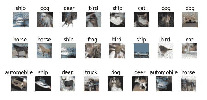 # 介紹 具有 10 個類別的 CIFAR 10 圖像數據集是 8000 萬個微型圖像數據集的標記子集。 這些圖像由 Alex Krizhevsky，Vinod Nair 和 Geoffrey Hinton 收集。 有關此數據集的完整詳細信息，請訪問[這里](https://www.cs.toronto.edu/~kriz/cifar.html)。 在 10 個類別中，總共有 60,000 個`32 x 32`彩色圖像，包括 50,000 個訓練圖像和 10,000 個測試圖像。 類別如下： ```py labels = ['airplane','automobile','bird','cat','deer','dog','frog','horse','ship','truck'] ``` 以下是這些類別的圖像的一些示例：  # 應用 首先，以下是設置所需的導入： ```py import tensorflow as tf import numpy as np from tensorflow.keras.datasets import cifar10 from tensorflow.keras.preprocessing.image import ImageDataGenerator from tensorflow.keras.models import Sequential from tensorflow.keras.layers import Dense, Dropout, Activation, Flatten from tensorflow.keras.layers import Conv2D, MaxPooling2D,BatchNormalization from tensorflow.keras import regularizers from tensorflow.keras.models import load_model import os from matplotlib import pyplot as plt from PIL import Image ``` 您可能需要運行`pip install PIL`。 接下來，我們將在其余的代碼中使用一組值： ```py batch_size = 32 number_of_classes = 10 epochs = 100 # for testing; use epochs = 100 for training ~30 secs/epoch on CPU weight_decay = 1e-4 save_dir = os.path.join(os.getcwd(), 'saved_models') model_name = 'keras_cifar10_trained_model.h5' number_of_images = 5 ``` 然后，我們可以加載并查看數據的形狀： ```py (x_train, y_train), (x_test, y_test) = cifar10.load_data() print('x_train shape:', x_train.shape) print(x_train.shape[0], 'train samples') print(x_test.shape[0], 'test samples') ``` 這將產生預期的輸出： ```py x_train shape: (50000, 32, 32, 3) 50000 train samples 10000 test samples ``` 現在，我們有了一個顯示圖像子集的函數。 這將在網格中顯示它們： ```py def show_images(images): plt.figure(1) image_index = 0 for i in range(0,number_of_images): for j in range(0,number_of_images): plt.subplot2grid((number_of_images, number_of_images),(i,j)) plt.imshow(Image.fromarray(images[image_index])) image_index +=1 plt.gca().axes.get_yaxis().set_visible(False) plt.gca().axes.get_xaxis().set_visible(False) plt.show() ``` 讓我們執行以下函數的調用： ```py show_images(x_test[:number_of_images*number_of_images]) ``` 這給我們以下輸出：  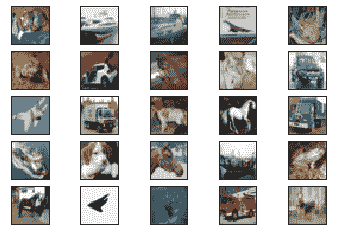請注意，圖像在原始數據集中故意很小。 現在，我們可以將圖像投射到浮動對象上，并將其范圍更改為`[0, 1]`： ```py x_train = x_train.astype('float32')/255 x_test = x_test.astype('float32')/255 ``` 如果將標簽作為一站式向量提供，則最好了解它們，因此，我們現在將這樣做： ```py y_train = tf.keras.utils.to_categorical(y_train, number_of_classes) # or use tf.one_hot() y_test = tf.keras.utils.to_categorical(y_test, number_of_classes) ``` 接下來，我們可以指定模型的架構。 請注意，與之前的操作相比，我們使用的激活指定方法略有不同： ```py model.add(Activation('elu')) ``` `elu`激活函數代表指數線性單元。 在[這個頁面](https://sefiks.com/2018/01/02/elu-as-a-neural-networks-activation-function/)中有很好的描述。 注意，我們正在使用具有卷積層，`BatchNormalization`和 MaxPooling 層的順序模型。 倒數第二層使結構變平，最后一層使用 softmax 激活，因此我們預測的類將顯示為具有最高激活的輸出神經元： ```py model = Sequential() model.add(Conv2D(32, (3,3), padding='same', kernel_regularizer=regularizers.l2(weight_decay), input_shape=x_train.shape[1:])) model.add(Activation('elu')) model.add(BatchNormalization()) model.add(Conv2D(32, (3,3), padding='same', kernel_regularizer=regularizers.l2(weight_decay))) model.add(Activation('elu')) model.add(BatchNormalization()) model.add(MaxPooling2D(pool_size=(2,2))) model.add(Dropout(0.2)) model.add(Conv2D(64, (3,3), padding='same', kernel_regularizer=regularizers.l2(weight_decay))) model.add(Activation('elu')) model.add(BatchNormalization()) model.add(Conv2D(64, (3,3), padding='same', kernel_regularizer=regularizers.l2(weight_decay))) model.add(Activation('elu')) model.add(BatchNormalization()) model.add(MaxPooling2D(pool_size=(2,2))) model.add(Dropout(0.3)) model.add(Conv2D(128, (3,3), padding='same', kernel_regularizer=regularizers.l2(weight_decay))) model.add(Activation('elu')) model.add(BatchNormalization()) model.add(Conv2D(128, (3,3), padding='same', kernel_regularizer=regularizers.l2(weight_decay))) model.add(Activation('elu')) model.add(BatchNormalization()) model.add(MaxPooling2D(pool_size=(2,2))) model.add(Dropout(0.4)) model.add(Flatten()) model.add(Dense(number_of_classes, activation='softmax')) ``` 接下來，我們必須定義我們的優化器； `RMSprop`。 `decay`是每次更新后學習率降低的速度： ```py opt = tf.keras.optimizers.RMSprop(lr=0.0001, decay=decay) ``` 現在，我們將編譯我們的模型： ```py model.compile(loss='categorical_crossentropy', optimizer=opt,metrics=['accuracy']) ``` 為了幫助模型學習和推廣，我們將實現實時數據增強。 這是通過`ImageDataGenerator()`函數完成的。 其簽名如下： ```py keras.preprocessing.image.ImageDataGenerator(featurewise_center=False, samplewise_center=False, featurewise_std_normalization=False, samplewise_std_normalization=False, zca_whitening=False, zca_epsilon=1e-06, rotation_range=0, width_shift_range=0.0, height_shift_range=0.0, brightness_range=None, shear_range=0.0, zoom_range=0.0, channel_shift_range=0.0, fill_mode='nearest', cval=0.0, horizontal_flip=False, vertical_flip=False, rescale=None, preprocessing_function=None, data_format=None, validation_split=0.0, dtype=None) ``` 但是，我們將主要使用前面簽名中所示的默認值。 數據將分批循環。 這是對圖像應用各種轉換，例如水平翻轉，高度偏移，寬度偏移，旋轉等。 我們將使用以下代碼進行演示： ```py # This will do preprocessing and real-time data augmentation: datagen = ImageDataGenerator( rotation_range=10, # randomly rotate images in the range 0 to 10 degrees width_shift_range=0.1,# randomly shift images horizontally (fraction of total width) height_shift_range=0.1,# randomly shift images vertically (fraction of total height) horizontal_flip=True, # randomly flip images validation_split=0.1) ``` 我們還將建立一個回調，以便如果模型的準確率停止提高，訓練將停止，并且將為模型恢復最佳權重。 `EarlyStopping`回調的簽名如下： ```py keras.callbacks.EarlyStopping(monitor='val_loss', min_delta=0, patience=0, verbose=0, mode='auto', baseline=None, restore_best_weights=False) ``` `Monitor`是要跟蹤的數量，`min_delta`是被算作改進的跟蹤數量的最小變化，`patience`是沒有變化的周期數，之后將停止訓練，而`mode` 是['min'，'max'，'auto']之一，它分別確定所跟蹤的值是應該減少還是增加，或者分別從其名稱中確定。 `baseline`是要達到的跟蹤值的值，而`restore_best_weights`確定是否應恢復最佳周期的模型權重（如果使用`false`，則使用最新權重）。 我們將有以下代碼： ```py callback = tf.keras.callbacks.EarlyStopping(monitor='accuracy', min_delta=0, patience=1, verbose=1,mode='max', restore_best_weights=True) ``` 現在，我們可以訓練模型了。 `fit.generator()`函數用于根據`flow()`生成器批量顯示的數據訓練模型。 可以在[這個頁面](https://keras.io/models/sequential/#fit_generator)中找到更多詳細信息： ```py model.fit_generator(datagen.flow(x_train, y_train, batch_size=batch_size), epochs=epochs, callbacks=[callback]) ``` 讓我們保存模型，以便以后可以重新加載它： ```py if not os.path.isdir(save_dir): os.makedirs(save_dir) model_path = os.path.join(save_dir, model_name) model.save(model_path) print('Model saved at: %s ' % model_path) ``` 現在讓我們重新加載它： ```py model1 = tf.keras.models.load_model(model_path) model1.summary() ``` 最后，讓我們看看我們的模型在測試集上的表現如何。 我們需要重新加載數據，因為它已被損壞： ```py (x_train, y_train), (x_test, y_test) = cifar10.load_data() show_images(x_test[:num_images*num_images]) x_test = x_test.astype('float32')/255 ``` 這里又是標簽： ```py labels = ['airplane','automobile','bird','cat','deer','dog','frog','horse','ship','truck'] ``` 最后，我們可以檢查預測的標簽： ```py indices = tf.argmax(input=model1.predict(x_test[:number_of_images*number_of_images]),axis=1) i = 0 print('Learned \t True') print('=====================') for index in indices: print(labels[index], '\t', labels[y_test[i][0]]) i+=1 ``` 在一次運行中，提前停止開始了 43 個周期，測試準確率為 81.4%，并且前 25 張圖像的測試結果如下： ```py Learned True ===================== cat cat ship ship ship ship ship airplane frog frog frog frog automobile automobile frog frog cat cat automobile automobile airplane airplane truck truck dog dog horse horse truck truck ship ship dog dog horse horse ship ship frog frog horse horse airplane airplane deer deer truck truck deer dog ``` 可以通過進一步調整模型架構和超參數（例如學習率）來提高此準確率。 到此結束了我們對 CIFAR 10 圖像數據集的了解。 # 總結 本章分為兩個部分。 在第一部分中，我們研究了來自 Google 的數據集 QuickDraw。 我們介紹了它，然后看到了如何將其加載到內存中。 這很簡單，因為 Google 善意地將數據集作為一組`.npy`文件提供，這些文件可以直接加載到 NumPy 數組中。 接下來，我們將數據分為訓練，驗證和測試集。 創建`ConvNet`模型后，我們對數據進行了訓練并進行了測試。 在測試中，經過 25 個周期，該模型的準確率剛好超過 90%，我們注意到，通過進一步調整模型，可能會改善這一精度。 最后，我們看到了如何保存經過訓練的模型，然后如何重新加載它并將其用于進一步的推斷。 在第二部分中，我們訓練了一個模型來識別 CIFAR 10 圖像數據集中的圖像。 該數據集包含 10 類圖像，是用于測試體系結構和進行超參數研究的流行數據集。 我們的準確率剛剛超過 81%。 在下一章中，我們將研究神經風格遷移，其中涉及獲取一個圖像的內容并將第二個圖像的風格強加于其上，以生成第三個混合圖像。