# 九、循環神經網絡 在本章中，我們將介紹循環神經網絡（RNN）以及如何在 TensorFlow 中實現它們。我們將首先演示如何使用 RNN 來預測垃圾郵件。然后，我們將介紹一種用于創建莎士比亞文本的 RNN 變體。我們將通過創建 RNN 序列到序列模型來完成從英語到德語的翻譯： * 實現 RNN 以進行垃圾郵件預測 * 實現 LSTM 模型 * 堆疊多個 LSTM 層 * 創建序列到序列模型 * 訓練 Siamese 相似性度量 本章的所有代碼都可以在 [Github](https://github.com/nfmcclure/tensorflow_cookbook) 和 [Packt 在線倉庫](https://github.com/PacktPublishing/TensorFlow-Machine-Learning-Cookbook-Second-Edition)。 # 介紹 在迄今為止我們考慮過的所有機器學習算法中，沒有人將數據視為序列。為了考慮序列數據，我們擴展了存儲先前迭代輸出的神經網絡。這種類型的神經網絡稱為 RNN。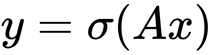考慮完全連接的網絡秘籍：  這里，權重由`A`乘以輸入層`x`給出，然后通過激活函數`σ`，給出輸出層`y`。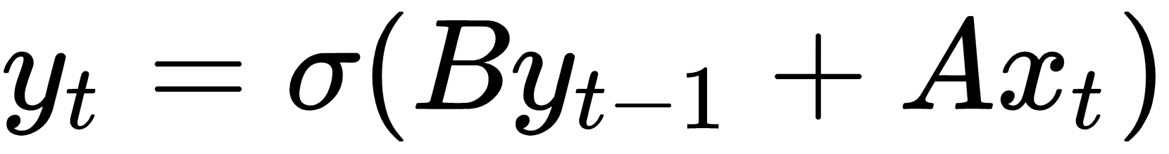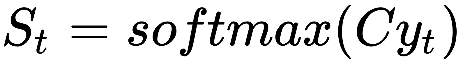 如果我們有一系列輸入數據`x[1], x[2], x[3], ...`，我們可以調整完全連接的層以考慮先前的輸入，如下所示：  在此循環迭代之上獲取下一個輸入，我們希望得到概率分布輸出，如下所示：  一旦我們有一個完整的序列輸出`{S[1], S[2], S[3], ...}`，我們可以通過考慮最后的輸出將目標視為數字或類別。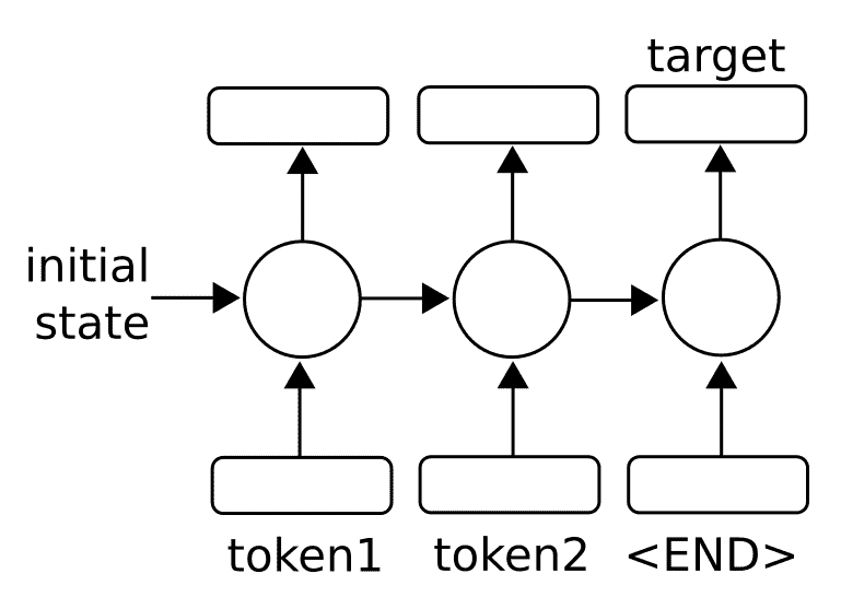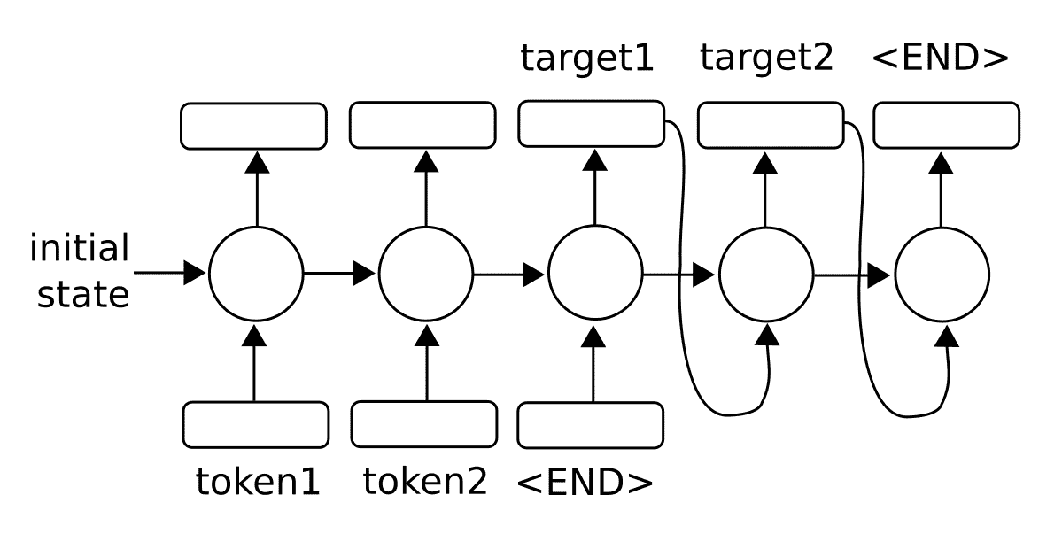有關通用架構的工作原理，請參見下圖：  圖 1：為了預測單個數字或類別，我們采用一系列輸入（標記）并將最終輸出視為預測輸出 我們還可以將序列輸出視為序列到序列模型中的輸入：  圖 2：為了預測序列，我們還可以將輸出反饋到模型中以生成多個輸出 對于任意長序列，使用反向傳播算法進行訓練會產生長時間相關的梯度。因此，存在消失或爆炸的梯度問題。在本章的后面，我們將通過將 RNN 單元擴展為所謂的長短期記憶（LSTM）單元來探索該問題的解決方案。主要思想是 LSTM 單元引入另一個操作，稱為門，它控制通過序列的信息流。我們將在后面的章節中詳細介紹。 > 在處理 NLP 的 RNN 模型時，編碼是用于描述將數據（NLP 中的字或字符）轉換為數字 RNN 特征的過程的術語。術語解碼是將 RNN 數字特征轉換為輸出字或字符的過程。 # 為垃圾郵件預測實現 RNN 首先，我們將應用標準 RNN 單元來預測奇異數值輸出，即垃圾郵件概率。 ## 準備 在此秘籍中，我們將在 TensorFlow 中實現標準 RNN，以預測短信是垃圾郵件還是非垃圾郵件。我們將使用 UCI 的 ML 倉庫中的 SMS 垃圾郵件收集數據集。我們將用于預測的架構將是來自嵌入文本的輸入 RNN 序列，我們將最后的 RNN 輸出作為垃圾郵件或非垃圾郵件（1 或 0）的預測。 ## 操作步驟 1. 我們首先加載此腳本所需的庫： ```py import os import re import io import requests import numpy as np import matplotlib.pyplot as plt import tensorflow as tf from zipfile import ZipFile ``` 1. 接下來，我們啟動圖會話并設置 RNN 模型參數。我們將通過`20`周期以`250`的批量大小運行數據。我們將考慮的每個文本的最大長度是`25`字；我們將更長的文本剪切為`25`或零填充短文本。 RNN 將是`10`單元。我們只考慮在詞匯表中出現至少 10 次的單詞，并且每個單詞都將嵌入到可訓練的大小`50`中。丟棄率將是我們可以在訓練期間`0.5`或評估期間`1.0`設置的占位符： ```py sess = tf.Session() epochs = 20 batch_size = 250 max_sequence_length = 25 rnn_size = 10 embedding_size = 50 min_word_frequency = 10 learning_rate = 0.0005 dropout_keep_prob = tf.placeholder(tf.float32) ``` 1. 現在我們獲取 SMS 文本數據。首先，我們檢查它是否已經下載，如果是，請在文件中讀取。否則，我們下載數據并保存： ```py data_dir = 'temp' data_file = 'text_data.txt' if not os.path.exists(data_dir): os.makedirs(data_dir) if not os.path.isfile(os.path.join(data_dir, data_file)): zip_url = 'http://archive.ics.uci.edu/ml/machine-learning-databases/00228/smsspamcollection.zip' r = requests.get(zip_url) z = ZipFile(io.BytesIO(r.content)) file = z.read('SMSSpamCollection') # Format Data text_data = file.decode() text_data = text_data.encode('ascii',errors='ignore') text_data = text_data.decode().split('\n') # Save data to text file with open(os.path.join(data_dir, data_file), 'w') as file_conn: for text in text_data: file_conn.write("{}\n".format(text)) else: # Open data from text file text_data = [] with open(os.path.join(data_dir, data_file), 'r') as file_conn: for row in file_conn: text_data.append(row) text_data = text_data[:-1] text_data = [x.split('\t') for x in text_data if len(x)>=1] [text_data_target, text_data_train] = [list(x) for x in zip(*text_data)] ``` 1. 為了減少我們的詞匯量，我們將通過刪除特殊字符和額外的空格來清理輸入文本，并將所有內容放在小寫中： ```py def clean_text(text_string): text_string = re.sub(r'([^sw]|_|[0-9])+', '', text_string) text_string = " ".join(text_string.split()) text_string = text_string.lower() return text_string # Clean texts text_data_train = [clean_text(x) for x in text_data_train] ``` > 請注意，我們的清潔步驟會刪除特殊字符作為替代方案，我們也可以用空格替換它們。理想情況下，這取決于數據集的格式。 1. 現在我們使用 TensorFlow 的內置詞匯處理器函數處理文本。這會將文本轉換為適當的索引列表： ```py vocab_processor = tf.contrib.learn.preprocessing.VocabularyProcessor(max_sequence_length, min_frequency=min_word_frequency) text_processed = np.array(list(vocab_processor.fit_transform(text_data_train))) ``` > 請注意，`contrib.learn.preprocessing`中的函數目前已棄用（使用當前的 TensorFlow 版本，1.10）。目前的替換建議 TensorFlow 預處理包僅在 Python2 中運行。將 TensorFlow 預處理移至 Python3 的工作目前正在進行中，并將取代前兩行。請記住，所有當前和最新的代碼都可以在[這個 GitHub 頁面](https://www.github.com/nfmcclure/tensorflow_cookbook)，和 [Packt 倉庫](https://github.com/PacktPublishing/TensorFlow-Machine-Learning-Cookbook-Second-Edition)找到。 1. 接下來，我們打亂數據以使其隨機化： ```py text_processed = np.array(text_processed) text_data_target = np.array([1 if x=='ham' else 0 for x in text_data_target]) shuffled_ix = np.random.permutation(np.arange(len(text_data_target))) x_shuffled = text_processed[shuffled_ix] y_shuffled = text_data_target[shuffled_ix] ``` 1. 我們還將數據拆分為 80-20 訓練測試數據集： ```py ix_cutoff = int(len(y_shuffled)*0.80) x_train, x_test = x_shuffled[:ix_cutoff], x_shuffled[ix_cutoff:] y_train, y_test = y_shuffled[:ix_cutoff], y_shuffled[ix_cutoff:] vocab_size = len(vocab_processor.vocabulary_) print("Vocabulary Size: {:d}".format(vocab_size)) print("80-20 Train Test split: {:d} -- {:d}".format(len(y_train), len(y_test))) ``` > 對于這個秘籍，我們不會進行任何超參數調整。如果讀者朝這個方向前進，請記住在繼續之前將數據集拆分為訓練測試驗證集。一個很好的選擇是 Scikit-learn 函數`model_selection.train_test_split()`。 1. 接下來，我們聲明圖占位符。`x`輸入將是一個大小為`[None, max_sequence_length]`的占位符，它將是根據文本消息允許的最大字長的批量大小。對于非垃圾郵件或垃圾郵件，`y_output`占位符只是一個 0 或 1 的整數： ```py x_data = tf.placeholder(tf.int32, [None, max_sequence_length]) y_output = tf.placeholder(tf.int32, [None]) ``` 1. 我們現在為`x`輸入數據創建嵌入矩陣和嵌入查找操作： ```py embedding_mat = tf.Variable(tf.random_uniform([vocab_size, embedding_size], -1.0, 1.0)) embedding_output = tf.nn.embedding_lookup(embedding_mat, x_data) ``` 1. 我們將模型聲明如下。首先，我們初始化一種要使用的 RNN 單元（RNN 大小為 10）。然后我們通過使其成為動態 RNN 來創建 RNN 序列。然后我們將退出添加到 RNN： ```py cell = tf.nn.rnn_cell.BasicRNNCell(num_units = rnn_size) output, state = tf.nn.dynamic_rnn(cell, embedding_output, dtype=tf.float32) output = tf.nn.dropout(output, dropout_keep_prob) ``` > 注意，動態 RNN 允許可變長度序列。即使我們在這個例子中使用固定的序列長度，通常最好在 TensorFlow 中使用`dynamic_rnn`有兩個主要原因。一個原因是，在實踐中，動態 RNN 實際上運行速度更快；第二個是，如果我們選擇，我們可以通過 RNN 運行不同長度的序列。 1. 現在要得到我們的預測，我們必須重新安排 RNN 并切掉最后一個輸出： ```py output = tf.transpose(output, [1, 0, 2]) last = tf.gather(output, int(output.get_shape()[0]) - 1) ``` 1. 為了完成 RNN 預測，我們通過完全連接的網絡層將`rnn_size`輸出轉換為兩個類別輸出： ```py weight = tf.Variable(tf.truncated_normal([rnn_size, 2], stddev=0.1)) bias = tf.Variable(tf.constant(0.1, shape=[2])) logits_out = tf.nn.softmax(tf.matmul(last, weight) + bias) ``` 1. 我們接下來宣布我們的損失函數。請記住，當使用 TensorFlow 中的`sparse_softmax`函數時，目標必須是整數索引（類型為`int`），并且對率必須是浮點數： ```py losses = tf.nn.sparse_softmax_cross_entropy_with_logits(logits=logits_out, labels=y_output) loss = tf.reduce_mean(losses) ``` 1. 我們還需要一個精確度函數，以便我們可以比較測試和訓練集上的算法： ```py accuracy = tf.reduce_mean(tf.cast(tf.equal(tf.argmax(logits_out, 1), tf.cast(y_output, tf.int64)), tf.float32)) ``` 1. 接下來，我們創建優化函數并初始化模型變量： ```py optimizer = tf.train.RMSPropOptimizer(learning_rate) train_step = optimizer.minimize(loss) init = tf.global_variables_initializer() sess.run(init) ``` 1. 現在我們可以開始循環遍歷數據并訓練模型。在多次循環數據時，最好在每個周期對數據進行洗牌以防止過度訓練： ```py train_loss = [] test_loss = [] train_accuracy = [] test_accuracy = [] # Start training for epoch in range(epochs): # Shuffle training data shuffled_ix = np.random.permutation(np.arange(len(x_train))) x_train = x_train[shuffled_ix] y_train = y_train[shuffled_ix] num_batches = int(len(x_train)/batch_size) + 1 for i in range(num_batches): # Select train data min_ix = i * batch_size max_ix = np.min([len(x_train), ((i+1) * batch_size)]) x_train_batch = x_train[min_ix:max_ix] y_train_batch = y_train[min_ix:max_ix] # Run train step train_dict = {x_data: x_train_batch, y_output: y_train_batch, dropout_keep_prob:0.5} sess.run(train_step, feed_dict=train_dict) # Run loss and accuracy for training temp_train_loss, temp_train_acc = sess.run([loss, accuracy], feed_dict=train_dict) train_loss.append(temp_train_loss) train_accuracy.append(temp_train_acc) # Run Eval Step test_dict = {x_data: x_test, y_output: y_test, dropout_keep_prob:1.0} temp_test_loss, temp_test_acc = sess.run([loss, accuracy], feed_dict=test_dict) test_loss.append(temp_test_loss) test_accuracy.append(temp_test_acc) print('Epoch: {}, Test Loss: {:.2}, Test Acc: {:.2}'.format(epoch+1, temp_test_loss, temp_test_acc)) ``` 1. 這產生以下輸出： ```py Vocabulary Size: 933 80-20 Train Test split: 4459 -- 1115 Epoch: 1, Test Loss: 0.59, Test Acc: 0.83 Epoch: 2, Test Loss: 0.58, Test Acc: 0.83 ... ``` ```py Epoch: 19, Test Loss: 0.46, Test Acc: 0.86 Epoch: 20, Test Loss: 0.46, Test Acc: 0.86 ``` 1. 以下是繪制訓練/測試損失和準確率的代碼： ```py epoch_seq = np.arange(1, epochs+1) plt.plot(epoch_seq, train_loss, 'k--', label='Train Set') plt.plot(epoch_seq, test_loss, 'r-', label='Test Set') plt.title('Softmax Loss') plt.xlabel('Epochs') plt.ylabel('Softmax Loss') plt.legend(loc='upper left') plt.show() # Plot accuracy over time plt.plot(epoch_seq, train_accuracy, 'k--', label='Train Set') plt.plot(epoch_seq, test_accuracy, 'r-', label='Test Set') plt.title('Test Accuracy') plt.xlabel('Epochs') plt.ylabel('Accuracy') plt.legend(loc='upper left') plt.show() ``` ## 工作原理 在這個秘籍中，我們創建了一個 RNN 到類別的模型來預測 SMS 文本是垃圾郵件還是非垃圾郵件。我們在測試裝置上實現了大約 86% 的準確率。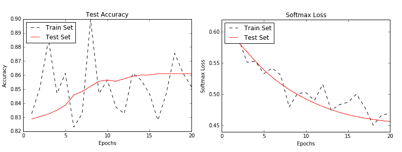以下是測試和訓練集的準確率和損失圖：  圖 3：訓練和測試集的準確率（左）和損失（右） ## 更多 強烈建議您多次瀏覽訓練數據集以獲取順序數據（這也建議用于非順序數據）。每次傳遞數據都稱為周期。此外，在每個周期之前對數據進行混洗是非常常見的（并且強烈推薦），以最小化數據順序對訓練的影響。 # 實現 LSTM 模型 我們將擴展我們的 RNN 模型，以便通過在此秘籍中引入 LSTM 單元來使用更長的序列。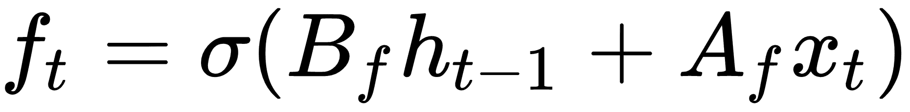 ## 準備 長短期記憶（LSTM）是傳統 RNN 的變體。 LSTM 是一種解決可變長度 RNN 所具有的消失/爆炸梯度問題的方法。為了解決這個問題，LSTM 單元引入了一個內部遺忘門，它可以修改從一個單元到下一個單元的信息流。為了概念化它的工作原理，我們將逐步介紹一個無偏置的 LSTM 方程式。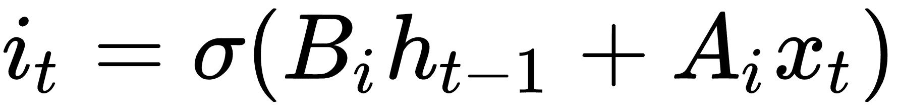第一步與常規 RNN 相同：  為了確定我們想要忘記或通過的值，我們將如下評估候選值。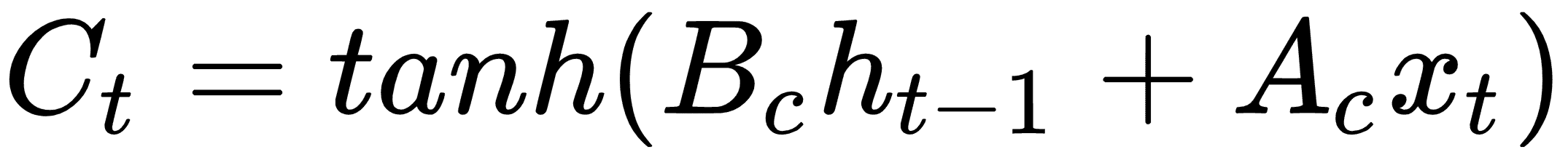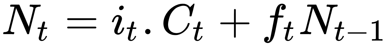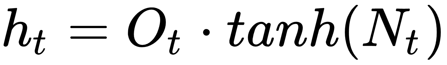這些值通常稱為存儲單元：  現在我們用一個遺忘矩陣修改候選存儲單元，其計算方法如下：  我們現在將遺忘存儲器與先前的存儲器步驟相結合，并將其添加到候選存儲器單元以獲得新的存儲器值：  現在我們將所有內容組合起來以獲取單元格的輸出：  然后，對于下一次迭代，我們更新`h`如下：  LSTM 的想法是通過基于輸入到單元的信息可以忘記或修改的單元具有自我調節的信息流。 > 在這里使用 TensorFlow 的一個好處是我們不必跟蹤這些操作及其相應的反向傳播屬性。 TensorFlow 將跟蹤這些并根據我們的損失函數，優化器和學習率指定的梯度自動更新模型變量。 對于這個秘籍，我們將使用具有 LSTM 單元的序列 RNN 來嘗試預測接下來的單詞，對莎士比亞的作品進行訓練。為了測試我們的工作方式，我們將提供模型候選短語，例如`thou art more`，并查看模型是否可以找出短語后面應該包含的單詞。 ## 操作步驟 1. 首先，我們為腳本加載必要的庫： ```py import os import re import string import requests import numpy as np import collections import random import pickle import matplotlib.pyplot as plt import tensorflow as tf ``` 1. 接下來，我們啟動圖會話并設置 RNN 參數： ```py sess = tf.Session() # Set RNN Parameters min_word_freq = 5 rnn_size = 128 epochs = 10 batch_size = 100 learning_rate = 0.001 training_seq_len = 50 embedding_size = rnn_size save_every = 500 eval_every = 50 prime_texts = ['thou art more', 'to be or not to', 'wherefore art thou'] ``` 1. 我們設置數據和模型文件夾和文件名，同時聲明要刪除的標點符號。我們希望保留連字符和撇號，因為莎士比亞經常使用它們來組合單詞和音節： ```py data_dir = 'temp' data_file = 'shakespeare.txt' model_path = 'shakespeare_model' full_model_dir = os.path.join(data_dir, model_path) # Declare punctuation to remove, everything except hyphens and apostrophe's punctuation = string.punctuation punctuation = ''.join([x for x in punctuation if x not in ['-', "'"]]) ``` 1. 接下來，我們獲取數據。如果數據文件不存在，我們下載并保存莎士比亞文本。如果確實存在，我們加載數據： ```py if not os.path.exists(full_model_dir): os.makedirs(full_model_dir) # Make data directory if not os.path.exists(data_dir): os.makedirs(data_dir) print('Loading Shakespeare Data') # Check if file is downloaded. if not os.path.isfile(os.path.join(data_dir, data_file)): print('Not found, downloading Shakespeare texts from www.gutenberg.org') shakespeare_url = 'http://www.gutenberg.org/cache/epub/100/pg100.txt' # Get Shakespeare text response = requests.get(shakespeare_url) shakespeare_file = response.content # Decode binary into string s_text = shakespeare_file.decode('utf-8') # Drop first few descriptive paragraphs. s_text = s_text[7675:] # Remove newlines s_text = s_text.replace('\r\n', '') s_text = s_text.replace('\n', '') # Write to file with open(os.path.join(data_dir, data_file), 'w') as out_conn: out_conn.write(s_text) else: # If file has been saved, load from that file with open(os.path.join(data_dir, data_file), 'r') as file_conn: s_text = file_conn.read().replace('\n', '') ``` 1. 我們通過刪除標點符號和額外的空格來清理莎士比亞的文本： ```py s_text = re.sub(r'[{}]'.format(punctuation), ' ', s_text) s_text = re.sub('s+', ' ', s_text ).strip().lower() ``` 1. 我們現在處理創建要使用的莎士比亞詞匯。我們創建一個函數，它將返回兩個字典（單詞到索引和索引到單詞），其中的單詞出現的頻率超過指定的頻率： ```py def build_vocab(text, min_word_freq): word_counts = collections.Counter(text.split(' ')) # limit word counts to those more frequent than cutoff word_counts = {key:val for key, val in word_counts.items() if val>min_word_freq} # Create vocab --> index mapping words = word_counts.keys() vocab_to_ix_dict = {key:(ix+1) for ix, key in enumerate(words)} # Add unknown key --> 0 index vocab_to_ix_dict['unknown']=0 # Create index --> vocab mapping ix_to_vocab_dict = {val:key for key,val in vocab_to_ix_dict.items()} return ix_to_vocab_dict, vocab_to_ix_dict ix2vocab, vocab2ix = build_vocab(s_text, min_word_freq) vocab_size = len(ix2vocab) + 1 ``` > 請注意，在處理文本時，我們必須小心索引值為零的單詞。我們應該保存填充的零值，也可能保存未知單詞。 1. 現在我們有了詞匯量，我們將莎士比亞的文本變成了一系列索引： ```py s_text_words = s_text.split(' ') s_text_ix = [] for ix, x in enumerate(s_text_words): try: s_text_ix.append(vocab2ix[x]) except: s_text_ix.append(0) s_text_ix = np.array(s_text_ix) ``` 1. 在本文中，我們將展示如何在類對象中創建模型。這對我們很有幫助，因為我們希望使用相同的模型（具有相同的權重）來批量訓練并從示例文本生成文本。如果沒有采用內部抽樣方法的類，這將很難做到。理想情況下，此類代碼應位于單獨的 Python 文件中，我們可以在此腳本的開頭導入該文件： ```py class LSTM_Model(): def __init__(self, rnn_size, batch_size, learning_rate, training_seq_len, vocab_size, infer =False): self.rnn_size = rnn_size self.vocab_size = vocab_size self.infer = infer self.learning_rate = learning_rate if infer: self.batch_size = 1 self.training_seq_len = 1 else: self.batch_size = batch_size self.training_seq_len = training_seq_len self.lstm_cell = tf.nn.rnn_cell.BasicLSTMCell(rnn_size) self.initial_state = self.lstm_cell.zero_state(self.batch_size, tf.float32) self.x_data = tf.placeholder(tf.int32, [self.batch_size, self.training_seq_len]) self.y_output = tf.placeholder(tf.int32, [self.batch_size, self.training_seq_len]) with tf.variable_scope('lstm_vars'): # Softmax Output Weights W = tf.get_variable('W', [self.rnn_size, self.vocab_size], tf.float32, tf.random_normal_initializer()) b = tf.get_variable('b', [self.vocab_size], tf.float32, tf.constant_initializer(0.0)) # Define Embedding embedding_mat = tf.get_variable('embedding_mat', [self.vocab_size, self.rnn_size], tf.float32, tf.random_normal_initializer()) embedding_output = tf.nn.embedding_lookup(embedding_mat, self.x_data) rnn_inputs = tf.split(embedding_output, num_or_size_splits=self.training_seq_len, axis=1) rnn_inputs_trimmed = [tf.squeeze(x, [1]) for x in rnn_inputs] # If we are inferring (generating text), we add a 'loop' function # Define how to get the i+1 th input from the i th output def inferred_loop(prev, count): prev_transformed = tf.matmul(prev, W) + b prev_symbol = tf.stop_gradient(tf.argmax(prev_transformed, 1)) output = tf.nn.embedding_lookup(embedding_mat, prev_symbol) return output decoder = tf.nn.seq2seq.rnn_decoder outputs, last_state = decoder(rnn_inputs_trimmed, self.initial_state, self.lstm_cell, loop_function=inferred_loop if infer else None) # Non inferred outputs output = tf.reshape(tf.concat(1, outputs), [-1, self.rnn_size]) # Logits and output self.logit_output = tf.matmul(output, W) + b self.model_output = tf.nn.softmax(self.logit_output) loss_fun = tf.contrib.legacy_seq2seq.sequence_loss_by_example loss = loss_fun([self.logit_output],[tf.reshape(self.y_output, [-1])], [tf.ones([self.batch_size * self.training_seq_len])], self.vocab_size) self.cost = tf.reduce_sum(loss) / (self.batch_size * self.training_seq_len) self.final_state = last_state gradients, _ = tf.clip_by_global_norm(tf.gradients(self.cost, tf.trainable_variables()), 4.5) optimizer = tf.train.AdamOptimizer(self.learning_rate) self.train_op = optimizer.apply_gradients(zip(gradients, tf.trainable_variables())) def sample(self, sess, words=ix2vocab, vocab=vocab2ix, num=10, prime_text='thou art'): state = sess.run(self.lstm_cell.zero_state(1, tf.float32)) word_list = prime_text.split() for word in word_list[:-1]: x = np.zeros((1, 1)) x[0, 0] = vocab[word] feed_dict = {self.x_data: x, self.initial_state:state} [state] = sess.run([self.final_state], feed_dict=feed_dict) out_sentence = prime_text word = word_list[-1] for n in range(num): x = np.zeros((1, 1)) x[0, 0] = vocab[word] feed_dict = {self.x_data: x, self.initial_state:state} [model_output, state] = sess.run([self.model_output, self.final_state], feed_dict=feed_dict) sample = np.argmax(model_output[0]) if sample == 0: break word = words[sample] out_sentence = out_sentence + ' ' + word return out_sentence ``` 1. 現在我們將聲明 LSTM 模型以及測試模型。我們將在變量范圍內執行此操作，并告訴范圍我們將重用測試 LSTM 模型的變量： ```py with tf.variable_scope('lstm_model', reuse=tf.AUTO_REUSE) as scope: # Define LSTM Model lstm_model = LSTM_Model(rnn_size, batch_size, learning_rate, training_seq_len, vocab_size) scope.reuse_variables() test_lstm_model = LSTM_Model(rnn_size, batch_size, learning_rate, training_seq_len, vocab_size, infer=True) ``` 1. 我們創建一個保存操作，并將輸入文本拆分為相等的批量大小的塊。然后我們初始化模型的變量： ```py saver = tf.train.Saver() # Create batches for each epoch num_batches = int(len(s_text_ix)/(batch_size * training_seq_len)) + 1 # Split up text indices into subarrays, of equal size batches = np.array_split(s_text_ix, num_batches) # Reshape each split into [batch_size, training_seq_len] batches = [np.resize(x, [batch_size, training_seq_len]) for x in batches] # Initialize all variables init = tf.global_variables_initializer() sess.run(init) ``` 1. 我們現在可以遍歷我們的周期，在每個周期開始之前對數據進行混洗。我們數據的目標只是相同的數據，但是移動了 1（使用`numpy.roll()`函數）： ```py train_loss = [] iteration_count = 1 for epoch in range(epochs): # Shuffle word indices random.shuffle(batches) # Create targets from shuffled batches targets = [np.roll(x, -1, axis=1) for x in batches] # Run a through one epoch print('Starting Epoch #{} of {}.'.format(epoch+1, epochs)) # Reset initial LSTM state every epoch state = sess.run(lstm_model.initial_state) for ix, batch in enumerate(batches): training_dict = {lstm_model.x_data: batch, lstm_model.y_output: targets[ix]} c, h = lstm_model.initial_state training_dict[c] = state.c training_dict[h] = state.h temp_loss, state, _ = sess.run([lstm_model.cost, lstm_model.final_state, lstm_model.train_op], feed_dict=training_dict) train_loss.append(temp_loss) # Print status every 10 gens if iteration_count % 10 == 0: summary_nums = (iteration_count, epoch+1, ix+1, num_batches+1, temp_loss) print('Iteration: {}, Epoch: {}, Batch: {} out of {}, Loss: {:.2f}'.format(*summary_nums)) # Save the model and the vocab if iteration_count % save_every == 0: # Save model model_file_name = os.path.join(full_model_dir, 'model') saver.save(sess, model_file_name, global_step = iteration_count) print('Model Saved To: {}'.format(model_file_name)) # Save vocabulary dictionary_file = os.path.join(full_model_dir, 'vocab.pkl') with open(dictionary_file, 'wb') as dict_file_conn: pickle.dump([vocab2ix, ix2vocab], dict_file_conn) if iteration_count % eval_every == 0: for sample in prime_texts: print(test_lstm_model.sample(sess, ix2vocab, vocab2ix, num=10, prime_text=sample)) iteration_count += 1 ``` 1. 這產生以下輸出： ```py Loading Shakespeare Data Cleaning Text Building Shakespeare Vocab Vocabulary Length = 8009 Starting Epoch #1 of 10\. Iteration: 10, Epoch: 1, Batch: 10 out of 182, Loss: 10.37 Iteration: 20, Epoch: 1, Batch: 20 out of 182, Loss: 9.54 ... Iteration: 1790, Epoch: 10, Batch: 161 out of 182, Loss: 5.68 Iteration: 1800, Epoch: 10, Batch: 171 out of 182, Loss: 6.05 thou art more than i am a to be or not to the man i have wherefore art thou art of the long Iteration: 1810, Epoch: 10, Batch: 181 out of 182, Loss: 5.99 ``` 1. 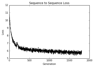最后，以下是我們如何繪制歷史上的訓練損失： ```py plt.plot(train_loss, 'k-') plt.title('Sequence to Sequence Loss') plt.xlabel('Generation') plt.ylabel('Loss') plt.show() ``` This results in the following plot of our loss values:  圖 4：模型所有代的序列到序列損失 ## 工作原理 在這個例子中，我們基于莎士比亞詞匯構建了一個帶有 LSTM 單元的 RNN 模型來預測下一個單詞。可以采取一些措施來改進模型，可能會增加序列大小，具有衰減的學習率，或者訓練模型以獲得更多的周期。 ## 更多 為了抽樣，我們實現了一個貪婪的采樣器。貪婪的采樣器可能會一遍又一遍地重復相同的短語；例如，他們可能會卡住`for the for the` `for the....`為了防止這種情況，我們還可以實現一種更隨機的采樣方式，可能是根據輸出的對數或概率分布制作加權采樣器。 # 堆疊多個 LSTM 層 正如我們可以增加神經網絡或 CNN 的深度，我們可以增加 RNN 網絡的深度。在這個秘籍中，我們應用了一個三層深度的 LSTM 來改進我們的莎士比亞語言生成。 ## 準備 我們可以通過將它們疊加在一起來增加循環神經網絡的深度。從本質上講，我們將獲取目標輸出并將其輸入另一個網絡。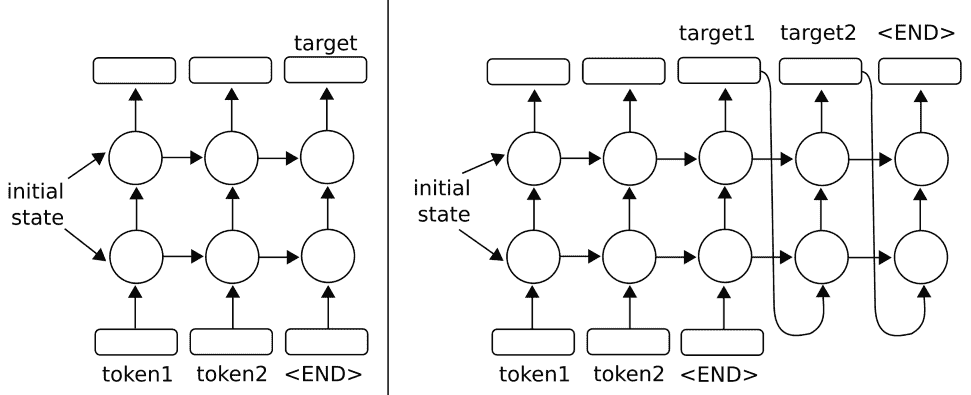 要了解這對于兩層的工作原理，請參見下圖：  圖 5：在上圖中，我們擴展了單層 RNN，使它們具有兩層。對于原始的單層版本，請參閱上一章簡介中的繪圖。左側架構說明了使用多層 RNN 預測輸出序列中的一個輸出的方法。正確的架構顯示了使用多層 RNN 預測輸出序列的方法，該輸出序列使用輸出作為輸入 TensorFlow 允許使用`MultiRNNCell()`函數輕松實現多個層，該函數接受 RNN 單元列表。有了這種行為，很容易用`MultiRNNCell([rnn_cell(num_units) for n in num_layers])`單元格從 Python 中的一個單元格創建多層 RNN。 對于這個秘籍，我們將執行我們在之前的秘籍中執行的相同的莎士比亞預測。將有兩個變化：第一個變化將是具有三個堆疊的 LSTM 模型而不是僅一個層，第二個變化將是進行字符級預測而不是單詞。進行字符級預測會將我們潛在的詞匯量大大減少到只有 40 個字符（26 個字母，10 個數字，1 個空格和 3 個特殊字符）。 ## 操作步驟 我們將說明本節中的代碼與上一節的不同之處，而不是重新使用所有相同的代碼。有關完整代碼，請參閱 [GitHub 倉庫](https://github.com/nfmcclure/tensorflow_cookbook)或 [Packt 倉庫](https://github.com/PacktPublishing/TensorFlow-Machine-Learning-Cookbook-Second-Edition)。 1. 我們首先需要設置模型的層數。我們將此作為參數放在腳本的開頭，并使用其他模型參數： ```py num_layers = 3 min_word_freq = 5 ``` ```py rnn_size = 128 epochs = 10 ``` 1. 第一個主要變化是我們將按字符加載，處理和提供文本，而不是按字詞加載。為了實現這一點，在清理文本之后，我們可以使用 Python 的`list()`命令逐個字符地分隔整個文本： ```py s_text = re.sub(r'[{}]'.format(punctuation), ' ', s_text) s_text = re.sub('s+', ' ', s_text ).strip().lower() # Split up by characters char_list = list(s_text) ``` 1. 我們現在需要更改 LSTM 模型，使其具有多個層。我們接受`num_layers`變量并使用 TensorFlow 的`MultiRNNCell()`函數創建一個多層 RNN 模型，如下所示： ```py class LSTM_Model(): def __init__(self, rnn_size, num_layers, batch_size, learning_rate, training_seq_len, vocab_size, infer_sample=False): self.rnn_size = rnn_size self.num_layers = num_layers self.vocab_size = vocab_size self.infer_sample = infer_sample self.learning_rate = learning_rate ... self.lstm_cell = tf.contrib.rnn.BasicLSTMCell(rnn_size) self.lstm_cell = tf.contrib.rnn.MultiRNNCell([self.lstm_cell for _ in range(self.num_layers)]) self.initial_state = self.lstm_cell.zero_state(self.batch_size, tf.float32) self.x_data = tf.placeholder(tf.int32, [self.batch_size, self.training_seq_len]) self.y_output = tf.placeholder(tf.int32, [self.batch_size, self.training_seq_len]) ``` > 請注意，TensorFlow 的`MultiRNNCell()`函數接受 RNN 單元列表。在這個項目中，RNN 層都是相同的，但您可以列出您希望堆疊在一起的任何 RNN 層。 1. 其他一切基本相同。在這里，我們可以看到一些訓練輸出： ```py Building Shakespeare Vocab by Characters Vocabulary Length = 40 Starting Epoch #1 of 10 Iteration: 9430, Epoch: 10, Batch: 889 out of 950, Loss: 1.54 Iteration: 9440, Epoch: 10, Batch: 899 out of 950, Loss: 1.46 Iteration: 9450, Epoch: 10, Batch: 909 out of 950, Loss: 1.49 thou art more than the to be or not to the serva wherefore art thou dost thou Iteration: 9460, Epoch: 10, Batch: 919 out of 950, Loss: 1.41 Iteration: 9470, Epoch: 10, Batch: 929 out of 950, Loss: 1.45 Iteration: 9480, Epoch: 10, Batch: 939 out of 950, Loss: 1.59 Iteration: 9490, Epoch: 10, Batch: 949 out of 950, Loss: 1.42 ``` 1. 以下是最終文本輸出的示例： ```py thou art more fancy with to be or not to be for be wherefore art thou art thou ``` 1. 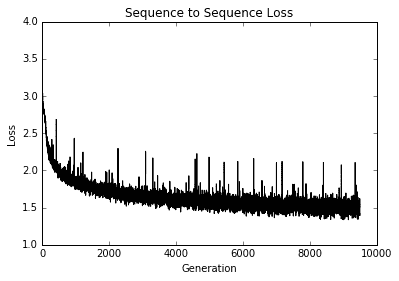最后，以下是我們如何繪制幾代的訓練損失： ```py plt.plot(train_loss, 'k-') plt.title('Sequence to Sequence Loss') plt.xlabel('Generation') plt.ylabel('Loss') plt.show() ```  圖 6：多層 LSTM 莎士比亞模型的訓練損失與世代的關系圖 ## 工作原理 TensorFlow 只需一個 RNN 單元列表即可輕松將 RNN 層擴展到多個層。對于這個秘籍，我們使用與上一個秘籍相同的莎士比亞數據，但是用字符而不是單詞處理它。我們通過三層 LSTM 模型來生成莎士比亞文本。我們可以看到，在僅僅 10 個周期之后，我們就能夠以文字的形式產生古老的英語。 # 創建序列到序列模型 由于我們使用的每個 RNN 單元也都有輸出，我們可以訓練 RNN 序列來預測其他可變長度的序列。對于這個秘籍，我們將利用這一事實創建一個英語到德語的翻譯模型。 ## 準備 對于這個秘籍，我們將嘗試構建一個語言翻譯模型，以便從英語翻譯成德語。 TensorFlow 具有用于序列到序列訓練的內置模型類。我們將說明如何在下載的英語 - 德語句子上訓練和使用它。我們將使用的數據來自 [www.manythings.org](http://www.manythings.org/) 的編譯 zip 文件，該文件匯編了 [Tatoeba 項目](http://tatoeba.org/home) 的數據。這些數據是制表符分隔的英語 - 德語句子翻譯；例如，一行可能包含句子`hello. /t hallo`。該數據包含數千種不同長度的句子。 此部分的代碼已升級為使用 [TensorFlow 官方倉庫提供的神經機器翻譯模型](https://github.com/tensorflow/nmt)。 該項目將向您展示如何下載數據，使用，修改和添加到超參數，以及配置您自己的數據以使用項目文件。 雖然官方教程向您展示了如何通過命令行執行此操作，但本教程將向您展示如何使用提供的內部代碼從頭開始訓練您自己的模型。 ## 操作步驟 1. 我們首先加載必要的庫： ```py import os import re import sys import json import math import time import string import requests import io import numpy as np import collections import random import pickle import string import matplotlib.pyplot as plt import tensorflow as tf from zipfile import ZipFile from collections import Counter from tensorflow.python.ops import lookup_ops from tensorflow.python.framework import ops ops.reset_default_graph() local_repository = 'temp/seq2seq' ``` 1. 以下代碼塊將整個 NMT 模型倉庫導入`temp`文件夾： ```py if not os.path.exists(local_repository): from git import Repo tf_model_repository = 'https://github.com/tensorflow/nmt/' Repo.clone_from(tf_model_repository, local_repository) sys.path.insert(0, 'temp/seq2seq/nmt/') # May also try to use 'attention model' by importing the attention model: # from temp.seq2seq.nmt import attention_model as attention_model from temp.seq2seq.nmt import model as model from temp.seq2seq.nmt.utils import vocab_utils as vocab_utils import temp.seq2seq.nmt.model_helper as model_helper import temp.seq2seq.nmt.utils.iterator_utils as iterator_utils import temp.seq2seq.nmt.utils.misc_utils as utils import temp.seq2seq.nmt.train as train ``` 1. 接下來，我們設置一些關于詞匯量大小，我們將刪除的標點符號以及數據存儲位置的參數： ```py # Model Parameters vocab_size = 10000 punct = string.punctuation # Data Parameters data_dir = 'temp' data_file = 'eng_ger.txt' model_path = 'seq2seq_model' full_model_dir = os.path.join(data_dir, model_path) ``` 1. 我們將使用 TensorFlow 提供的超參數格式。這種類型的參數存儲（在外部`json`或`xml`文件中）允許我們以編程方式迭代不同類型的架構（在不同的文件中）。對于本演示，我們將使用提供給我們的`wmt16.json`并進行一些更改： ```py # Load hyper-parameters for translation model. (Good defaults are provided in Repository). hparams = tf.contrib.training.HParams() param_file = 'temp/seq2seq/nmt/standard_hparams/wmt16.json' # Can also try: (For different architectures) # 'temp/seq2seq/nmt/standard_hparams/iwslt15.json' # 'temp/seq2seq/nmt/standard_hparams/wmt16_gnmt_4_layer.json', # 'temp/seq2seq/nmt/standard_hparams/wmt16_gnmt_8_layer.json', with open(param_file, "r") as f: params_json = json.loads(f.read()) for key, value in params_json.items(): hparams.add_hparam(key, value) hparams.add_hparam('num_gpus', 0) hparams.add_hparam('num_encoder_layers', hparams.num_layers) hparams.add_hparam('num_decoder_layers', hparams.num_layers) hparams.add_hparam('num_encoder_residual_layers', 0) hparams.add_hparam('num_decoder_residual_layers', 0) hparams.add_hparam('init_op', 'uniform') hparams.add_hparam('random_seed', None) hparams.add_hparam('num_embeddings_partitions', 0) hparams.add_hparam('warmup_steps', 0) hparams.add_hparam('length_penalty_weight', 0) hparams.add_hparam('sampling_temperature', 0.0) hparams.add_hparam('num_translations_per_input', 1) hparams.add_hparam('warmup_scheme', 't2t') hparams.add_hparam('epoch_step', 0) hparams.num_train_steps = 5000 # Not use any pretrained embeddings hparams.add_hparam('src_embed_file', '') hparams.add_hparam('tgt_embed_file', '') hparams.add_hparam('num_keep_ckpts', 5) hparams.add_hparam('avg_ckpts', False) # Remove attention hparams.attention = None ``` 1. 如果模型和數據目錄尚不存在，請創建它們： ```py # Make Model Directory if not os.path.exists(full_model_dir): os.makedirs(full_model_dir) # Make data directory if not os.path.exists(data_dir): os.makedirs(data_dir) ``` 1. 現在我們刪除標點符號并將翻譯數據拆分為英語和德語句子的單詞列表： ```py print('Loading English-German Data') # Check for data, if it doesn't exist, download it and save it if not os.path.isfile(os.path.join(data_dir, data_file)): print('Data not found, downloading Eng-Ger sentences from www.manythings.org') sentence_url = 'http://www.manythings.org/anki/deu-eng.zip' r = requests.get(sentence_url) z = ZipFile(io.BytesIO(r.content)) file = z.read('deu.txt') # Format Data eng_ger_data = file.decode('utf-8') eng_ger_data = eng_ger_data.encode('ascii', errors='ignore') eng_ger_data = eng_ger_data.decode().split('\n') # Write to file with open(os.path.join(data_dir, data_file), 'w') as out_conn: for sentence in eng_ger_data: out_conn.write(sentence + '\n') else: eng_ger_data = [] with open(os.path.join(data_dir, data_file), 'r') as in_conn: for row in in_conn: eng_ger_data.append(row[:-1]) print('Done!') ``` 1. 現在我們刪除英語和德語句子的標點符號： ```py # Remove punctuation eng_ger_data = [''.join(char for char in sent if char not in punct) for sent in eng_ger_data] # Split each sentence by tabs eng_ger_data = [x.split('\t') for x in eng_ger_data if len(x) >= 1] [english_sentence, german_sentence] = [list(x) for x in zip(*eng_ger_data)] english_sentence = [x.lower().split() for x in english_sentence] german_sentence = [x.lower().split() for x in german_sentence] ``` 1. 為了使用 TensorFlow 中更快的數據管道函數，我們需要以適當的格式將格式化的數據寫入磁盤。翻譯模型期望的格式如下： ```py train_prefix.source_suffix = train.en train_prefix.target_suffix = train.de ``` 后綴將決定語言（`en = English`，`de = deutsch`），前綴決定數據集的類型（訓練或測試）： ```py # We need to write them to separate text files for the text-line-dataset operations. train_prefix = 'train' src_suffix = 'en' # English tgt_suffix = 'de' # Deutsch (German) source_txt_file = train_prefix + '.' + src_suffix hparams.add_hparam('src_file', source_txt_file) target_txt_file = train_prefix + '.' + tgt_suffix hparams.add_hparam('tgt_file', target_txt_file) with open(source_txt_file, 'w') as f: for sent in english_sentence: f.write(' '.join(sent) + '\n') with open(target_txt_file, 'w') as f: for sent in german_sentence: f.write(' '.join(sent) + '\n') ``` 1. 接下來，我們需要解析一些（~100）測試句子翻譯。我們任意選擇大約 100 個句子。然后我們也將它們寫入適當的文件： ```py # Partition some sentences off for testing files test_prefix = 'test_sent' hparams.add_hparam('dev_prefix', test_prefix) hparams.add_hparam('train_prefix', train_prefix) hparams.add_hparam('test_prefix', test_prefix) hparams.add_hparam('src', src_suffix) hparams.add_hparam('tgt', tgt_suffix) num_sample = 100 total_samples = len(english_sentence) # Get around 'num_sample's every so often in the src/tgt sentences ix_sample = [x for x in range(total_samples) if x % (total_samples // num_sample) == 0] test_src = [' '.join(english_sentence[x]) for x in ix_sample] test_tgt = [' '.join(german_sentence[x]) for x in ix_sample] # Write test sentences to file with open(test_prefix + '.' + src_suffix, 'w') as f: for eng_test in test_src: f.write(eng_test + '\n') with open(test_prefix + '.' + tgt_suffix, 'w') as f: for ger_test in test_src: f.write(ger_test + '\n') ``` 1. 接下來，我們處理英語和德語句子的詞匯表。然后我們將詞匯表列表保存到適當的文件中： ```py print('Processing the vocabularies.') # Process the English Vocabulary all_english_words = [word for sentence in english_sentence for word in sentence] all_english_counts = Counter(all_english_words) eng_word_keys = [x[0] for x in all_english_counts.most_common(vocab_size-3)] # -3 because UNK, S, /S is also in there eng_vocab2ix = dict(zip(eng_word_keys, range(1, vocab_size))) eng_ix2vocab = {val: key for key, val in eng_vocab2ix.items()} english_processed = [] for sent in english_sentence: temp_sentence = [] for word in sent: try: temp_sentence.append(eng_vocab2ix[word]) except KeyError: temp_sentence.append(0) english_processed.append(temp_sentence) # Process the German Vocabulary all_german_words = [word for sentence in german_sentence for word in sentence] all_german_counts = Counter(all_german_words) ger_word_keys = [x[0] for x in all_german_counts.most_common(vocab_size-3)] # -3 because UNK, S, /S is also in there ger_vocab2ix = dict(zip(ger_word_keys, range(1, vocab_size))) ger_ix2vocab = {val: key for key, val in ger_vocab2ix.items()} german_processed = [] for sent in german_sentence: temp_sentence = [] for word in sent: try: temp_sentence.append(ger_vocab2ix[word]) except KeyError: temp_sentence.append(0) german_processed.append(temp_sentence) # Save vocab files for data processing source_vocab_file = 'vocab' + '.' + src_suffix hparams.add_hparam('src_vocab_file', source_vocab_file) eng_word_keys = ['<unk>', '<s>', '</s>'] + eng_word_keys target_vocab_file = 'vocab' + '.' + tgt_suffix hparams.add_hparam('tgt_vocab_file', target_vocab_file) ger_word_keys = ['<unk>', '<s>', '</s>'] + ger_word_keys # Write out all unique english words with open(source_vocab_file, 'w') as f: for eng_word in eng_word_keys: f.write(eng_word + '\n') # Write out all unique german words with open(target_vocab_file, 'w') as f: for ger_word in ger_word_keys: f.write(ger_word + '\n') # Add vocab size to hyper parameters hparams.add_hparam('src_vocab_size', vocab_size) hparams.add_hparam('tgt_vocab_size', vocab_size) # Add out-directory out_dir = 'temp/seq2seq/nmt_out' hparams.add_hparam('out_dir', out_dir) if not tf.gfile.Exists(out_dir): tf.gfile.MakeDirs(out_dir) ``` 1. 接下來，我們將分別創建訓練，推斷和評估圖。首先，我們創建訓練圖。我們用一個類來做這個并將參數設為`namedtuple`。此代碼來自 NMT TensorFlow 倉庫。有關更多信息，請參閱名為`model_helper.py`的倉庫中的文件： ```py class TrainGraph(collections.namedtuple("TrainGraph", ("graph", "model", "iterator", "skip_count_placeholder"))): pass def create_train_graph(scope=None): graph = tf.Graph() with graph.as_default(): src_vocab_table, tgt_vocab_table = vocab_utils.create_vocab_tables(hparams.src_vocab_file, hparams.tgt_vocab_file,share_vocab=False) src_dataset = tf.data.TextLineDataset(hparams.src_file) tgt_dataset = tf.data.TextLineDataset(hparams.tgt_file) skip_count_placeholder = tf.placeholder(shape=(), dtype=tf.int64) iterator = iterator_utils.get_iterator(src_dataset, tgt_dataset, src_vocab_table, tgt_vocab_table, batch_size=hparams.batch_size, sos=hparams.sos, eos=hparams.eos, random_seed=None, num_buckets=hparams.num_buckets, src_max_len=hparams.src_max_len, tgt_max_len=hparams.tgt_max_len, skip_count=skip_count_placeholder) final_model = model.Model(hparams, iterator=iterator, mode=tf.contrib.learn.ModeKeys.TRAIN, source_vocab_table=src_vocab_table, target_vocab_table=tgt_vocab_table, scope=scope) return TrainGraph(graph=graph, model=final_model, iterator=iterator, skip_count_placeholder=skip_count_placeholder) train_graph = create_train_graph() ``` 1. 我們現在創建評估圖： ```py # Create the evaluation graph class EvalGraph(collections.namedtuple("EvalGraph", ("graph", "model", "src_file_placeholder", "tgt_file_placeholder","iterator"))): pass def create_eval_graph(scope=None): graph = tf.Graph() with graph.as_default(): src_vocab_table, tgt_vocab_table = vocab_utils.create_vocab_tables( hparams.src_vocab_file, hparams.tgt_vocab_file, hparams.share_vocab) src_file_placeholder = tf.placeholder(shape=(), dtype=tf.string) tgt_file_placeholder = tf.placeholder(shape=(), dtype=tf.string) src_dataset = tf.data.TextLineDataset(src_file_placeholder) tgt_dataset = tf.data.TextLineDataset(tgt_file_placeholder) iterator = iterator_utils.get_iterator( src_dataset, tgt_dataset, src_vocab_table, tgt_vocab_table, hparams.batch_size, sos=hparams.sos, eos=hparams.eos, random_seed=hparams.random_seed, num_buckets=hparams.num_buckets, src_max_len=hparams.src_max_len_infer, tgt_max_len=hparams.tgt_max_len_infer) final_model = model.Model(hparams, iterator=iterator, mode=tf.contrib.learn.ModeKeys.EVAL, source_vocab_table=src_vocab_table, target_vocab_table=tgt_vocab_table, scope=scope) return EvalGraph(graph=graph, model=final_model, src_file_placeholder=src_file_placeholder, tgt_file_placeholder=tgt_file_placeholder, iterator=iterator) eval_graph = create_eval_graph() ``` 1. 現在我們對推理圖做同樣的事情： ```py # Inference graph class InferGraph(collections.namedtuple("InferGraph", ("graph","model","src_placeholder", "batch_size_placeholder","iterator"))): pass def create_infer_graph(scope=None): graph = tf.Graph() with graph.as_default(): src_vocab_table, tgt_vocab_table = vocab_utils.create_vocab_tables(hparams.src_vocab_file,hparams.tgt_vocab_file, hparams.share_vocab) reverse_tgt_vocab_table = lookup_ops.index_to_string_table_from_file(hparams.tgt_vocab_file, default_value=vocab_utils.UNK) src_placeholder = tf.placeholder(shape=[None], dtype=tf.string) batch_size_placeholder = tf.placeholder(shape=[], dtype=tf.int64) src_dataset = tf.data.Dataset.from_tensor_slices(src_placeholder) iterator = iterator_utils.get_infer_iterator(src_dataset, src_vocab_table, batch_size=batch_size_placeholder, eos=hparams.eos, src_max_len=hparams.src_max_len_infer) final_model = model.Model(hparams, iterator=iterator, mode=tf.contrib.learn.ModeKeys.INFER, source_vocab_table=src_vocab_table, target_vocab_table=tgt_vocab_table, reverse_target_vocab_table=reverse_tgt_vocab_table, scope=scope) return InferGraph(graph=graph, model=final_model, src_placeholder=src_placeholder, batch_size_placeholder=batch_size_placeholder, iterator=iterator) infer_graph = create_infer_graph() ``` 1. 為了在訓練期間提供更多說明性輸出，我們提供了在訓練迭代期間輸出的任意源/目標翻譯的簡短列表： ```py # Create sample data for evaluation sample_ix = [25, 125, 240, 450] sample_src_data = [' '.join(english_sentence[x]) for x in sample_ix] sample_tgt_data = [' '.join(german_sentence[x]) for x in sample_ix] print([x for x in zip(sample_src_data, sample_tgt_data)]) ``` 1. 接下來，我們加載訓練圖： ```py config_proto = utils.get_config_proto() train_sess = tf.Session(config=config_proto, graph=train_graph.graph) eval_sess = tf.Session(config=config_proto, graph=eval_graph.graph) infer_sess = tf.Session(config=config_proto, graph=infer_graph.graph) # Load the training graph with train_graph.graph.as_default(): loaded_train_model, global_step = model_helper.create_or_load_model(train_graph.model, hparams.out_dir, train_sess, "train") summary_writer = tf.summary.FileWriter(os.path.join(hparams.out_dir, 'Training'), train_graph.graph) ``` 1. 現在我們將評估操作添加到圖中： ```py for metric in hparams.metrics: hparams.add_hparam("best_" + metric, 0) best_metric_dir = os.path.join(hparams.out_dir, "best_" + metric) hparams.add_hparam("best_" + metric + "_dir", best_metric_dir) tf.gfile.MakeDirs(best_metric_dir) eval_output = train.run_full_eval(hparams.out_dir, infer_graph, infer_sess, eval_graph, eval_sess, hparams, summary_writer, sample_src_data, sample_tgt_data) eval_results, _, acc_blue_scores = eval_output ``` 1. 現在我們創建初始化操作并初始化圖；我們還初始化了一些將更新每次迭代的參數（時間，全局步驟和周期步驟）： ```py # Training Initialization last_stats_step = global_step last_eval_step = global_step last_external_eval_step = global_step steps_per_eval = 10 * hparams.steps_per_stats steps_per_external_eval = 5 * steps_per_eval avg_step_time = 0.0 step_time, checkpoint_loss, checkpoint_predict_count = 0.0, 0.0, 0.0 checkpoint_total_count = 0.0 speed, train_ppl = 0.0, 0.0 utils.print_out("# Start step %d, lr %g, %s" % (global_step, loaded_train_model.learning_rate.eval(session=train_sess), time.ctime())) skip_count = hparams.batch_size * hparams.epoch_step utils.print_out("# Init train iterator, skipping %d elements" % skip_count) train_sess.run(train_graph.iterator.initializer, feed_dict={train_graph.skip_count_placeholder: skip_count}) ``` > 請注意，默認情況下，訓練將每 1,000 次迭代保存模型。如果需要，您可以在超參數中更改此設置。目前，訓練此模型并保存最新的五個模型占用大約 2 GB 的硬盤空間。 1. 以下代碼將開始模型的訓練和評估。訓練的重要部分是在循環的最開始（前三分之一）。其余代碼專門用于評估，從樣本推斷和保存模型，如下所示： ```py # Run training while global_step < hparams.num_train_steps: start_time = time.time() try: step_result = loaded_train_model.train(train_sess) (_, step_loss, step_predict_count, step_summary, global_step, step_word_count, batch_size, __, ___) = step_result hparams.epoch_step += 1 except tf.errors.OutOfRangeError: # Next Epoch hparams.epoch_step = 0 utils.print_out("# Finished an epoch, step %d. Perform external evaluation" % global_step) train.run_sample_decode(infer_graph, infer_sess, hparams.out_dir, hparams, summary_writer, sample_src_data, sample_tgt_data) dev_scores, test_scores, _ = train.run_external_eval(infer_graph, infer_sess, hparams.out_dir, hparams, summary_writer) train_sess.run(train_graph.iterator.initializer, feed_dict={train_graph.skip_count_placeholder: 0}) continue summary_writer.add_summary(step_summary, global_step) # Statistics step_time += (time.time() - start_time) checkpoint_loss += (step_loss * batch_size) checkpoint_predict_count += step_predict_count checkpoint_total_count += float(step_word_count) # print statistics if global_step - last_stats_step >= hparams.steps_per_stats: last_stats_step = global_step avg_step_time = step_time / hparams.steps_per_stats train_ppl = utils.safe_exp(checkpoint_loss / checkpoint_predict_count) speed = checkpoint_total_count / (1000 * step_time) utils.print_out(" global step %d lr %g " "step-time %.2fs wps %.2fK ppl %.2f %s" % (global_step, loaded_train_model.learning_rate.eval(session=train_sess), avg_step_time, speed, train_ppl, train._get_best_results(hparams))) if math.isnan(train_ppl): break # Reset timer and loss. step_time, checkpoint_loss, checkpoint_predict_count = 0.0, 0.0, 0.0 checkpoint_total_count = 0.0 if global_step - last_eval_step >= steps_per_eval: last_eval_step = global_step utils.print_out("# Save eval, global step %d" % global_step) utils.add_summary(summary_writer, global_step, "train_ppl", train_ppl) # Save checkpoint loaded_train_model.saver.save(train_sess, os.path.join(hparams.out_dir, "translate.ckpt"), global_step=global_step) # Evaluate on dev/test train.run_sample_decode(infer_graph, infer_sess, out_dir, hparams, summary_writer, sample_src_data, sample_tgt_data) dev_ppl, test_ppl = train.run_internal_eval(eval_graph, eval_sess, out_dir, hparams, summary_writer) if global_step - last_external_eval_step >= steps_per_external_eval: last_external_eval_step = global_step # Save checkpoint loaded_train_model.saver.save(train_sess, os.path.join(hparams.out_dir, "translate.ckpt"), global_step=global_step) train.run_sample_decode(infer_graph, infer_sess, out_dir, hparams, summary_writer, sample_src_data, sample_tgt_data) dev_scores, test_scores, _ = train.run_external_eval(infer_graph, infer_sess, out_dir, hparams, summary_writer) ``` ## 工作原理 對于這個秘籍，我們使用 TensorFlow 內置的序列到序列模型從英語翻譯成德語。 由于我們沒有為我們的測試句子提供完美的翻譯，因此還有改進的余地。如果我們訓練時間更長，并且可能組合一些桶（每個桶中有更多的訓練數據），我們可能能夠改進我們的翻譯。 ## 更多 在 ManyThings 網站上托管了其他類似的[雙語句子數據集](http://www.manythings.org/anki/)。您可以隨意替換任何吸引您的語言數據集。 # 訓練 Siamese RNN 相似性度量 與許多其他模型相比，RNN 模型的一個重要特性是它們可以處理各種長度的序列。利用這一點，以及它們可以推廣到之前未見過的序列這一事實，我們可以創建一種方法來衡量輸入的相似序列是如何相互作用的。在這個秘籍中，我們將訓練一個 Siamese 相似性 RNN 來測量地址之間的相似性以進行記錄匹配。 ## 準備 在本文中，我們將構建一個雙向 RNN 模型，該模型將輸入到一個完全連接的層，該層輸出一個固定長度的數值向量。我們為兩個輸入地址創建雙向 RNN 層，并將輸出饋送到完全連接的層，該層輸出固定長度的數字向量（長度 100）。然后我們將兩個向量輸出與余弦距離進行比較，余弦距離在 -1 和 1 之間。我們將輸入數據表示為與目標 1 相似，并且目標為 -1。余弦距離的預測只是輸出的符號（負值表示不相似，正表示相似）。我們可以使用此網絡通過從查詢地址獲取在余弦距離上得分最高的參考地址來進行記錄匹配。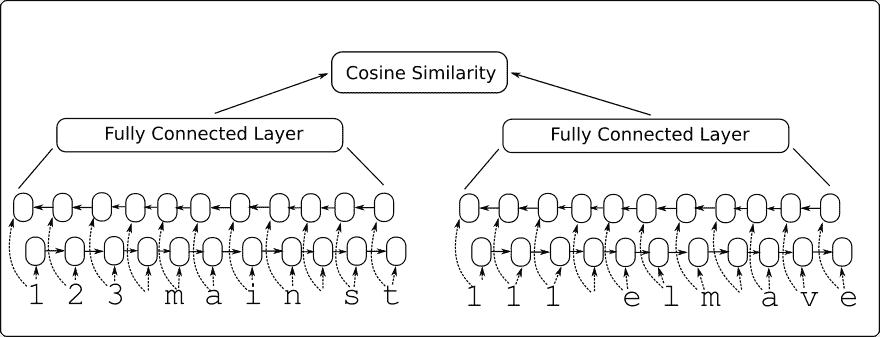 請參閱以下網絡架構圖：  圖 8：Siamese RNN 相似性模型架構 這個模型的優點還在于它接受以前沒有見過的輸入，并且可以將它們與 -1 到 1 的輸出進行比較。我們將通過選擇模型之前未見過的測試地址在代碼中顯示它并查看它是否可以匹配到類似的地址。 ## 操作步驟 1. 我們首先加載必要的庫并啟動圖會話： ```py import os import random import string import numpy as np import matplotlib.pyplot as plt import tensorflow as tf sess = tf.Session() ``` 1. 我們現在設置模型參數如下： ```py batch_size = 200 n_batches = 300 max_address_len = 20 margin = 0.25 num_features = 50 dropout_keep_prob = 0.8 ``` 1. 接下來，我們創建 Siamese RNN 相似性模型類，如下所示： ```py def snn(address1, address2, dropout_keep_prob, vocab_size, num_features, input_length): # Define the Siamese double RNN with a fully connected layer at the end def Siamese_nn(input_vector, num_hidden): cell_unit = tf.nn.rnn_cell.BasicLSTMCell # Forward direction cell lstm_forward_cell = cell_unit(num_hidden, forget_bias=1.0) lstm_forward_cell = tf.nn.rnn_cell.DropoutWrapper(lstm_forward_cell, output_keep_prob=dropout_keep_prob) # Backward direction cell lstm_backward_cell = cell_unit(num_hidden, forget_bias=1.0) lstm_backward_cell = tf.nn.rnn_cell.DropoutWrapper(lstm_backward_cell, output_keep_prob=dropout_keep_prob) # Split title into a character sequence input_embed_split = tf.split(1, input_length, input_vector) input_embed_split = [tf.squeeze(x, squeeze_dims=[1]) for x in input_embed_split] # Create bidirectional layer outputs, _, _ = tf.nn.bidirectional_rnn(lstm_forward_cell, lstm_backward_cell, input_embed_split, dtype=tf.float32) # Average The output over the sequence temporal_mean = tf.add_n(outputs) / input_length # Fully connected layer output_size = 10 A = tf.get_variable(name="A", shape=[2*num_hidden, output_size], dtype=tf.float32, initializer=tf.random_normal_initializer(stddev=0.1)) b = tf.get_variable(name="b", shape=[output_size], dtype=tf.float32, initializer=tf.random_normal_initializer(stddev=0.1)) final_output = tf.matmul(temporal_mean, A) + b final_output = tf.nn.dropout(final_output, dropout_keep_prob) return(final_output) with tf.variable_scope("Siamese") as scope: output1 = Siamese_nn(address1, num_features) # Declare that we will use the same variables on the second string scope.reuse_variables() output2 = Siamese_nn(address2, num_features) # Unit normalize the outputs output1 = tf.nn.l2_normalize(output1, 1) output2 = tf.nn.l2_normalize(output2, 1) # Return cosine distance # in this case, the dot product of the norms is the same. dot_prod = tf.reduce_sum(tf.mul(output1, output2), 1) return dot_prod ``` > 請注意，使用變量范圍在兩個地址輸入的 Siamese 網絡的兩個部分之間共享參數。另外，請注意，余弦距離是通過歸一化向量的點積來實現的。 1. 現在我們將聲明我們的預測函數，它只是余弦距離的符號，如下所示： ```py def get_predictions(scores): predictions = tf.sign(scores, name="predictions") return predictions ``` 1. 現在我們將如前所述聲明我們的`loss`函數。請記住，我們希望為誤差留下邊距（類似于 SVM 模型）。我們還將有一個真正的積極和真正的消極的損失期限。使用以下代碼進行損失： ```py def loss(scores, y_target, margin): # Calculate the positive losses pos_loss_term = 0.25 * tf.square(tf.sub(1., scores)) pos_mult = tf.cast(y_target, tf.float32) # Make sure positive losses are on similar strings positive_loss = tf.mul(pos_mult, pos_loss_term) # Calculate negative losses, then make sure on dissimilar strings neg_mult = tf.sub(1., tf.cast(y_target, tf.float32)) negative_loss = neg_mult*tf.square(scores) # Combine similar and dissimilar losses loss = tf.add(positive_loss, negative_loss) # Create the margin term. This is when the targets are 0, and the scores are less than m, return 0\. # Check if target is zero (dissimilar strings) target_zero = tf.equal(tf.cast(y_target, tf.float32), 0.) # Check if cosine outputs is smaller than margin less_than_margin = tf.less(scores, margin) # Check if both are true both_logical = tf.logical_and(target_zero, less_than_margin) both_logical = tf.cast(both_logical, tf.float32) # If both are true, then multiply by (1-1)=0\. multiplicative_factor = tf.cast(1\. - both_logical, tf.float32) total_loss = tf.mul(loss, multiplicative_factor) # Average loss over batch avg_loss = tf.reduce_mean(total_loss) return avg_loss ``` 1. 我們聲明`accuracy`函數如下： ```py def accuracy(scores, y_target): predictions = get_predictions(scores) correct_predictions = tf.equal(predictions, y_target) accuracy = tf.reduce_mean(tf.cast(correct_predictions, tf.float32)) return accuracy ``` 1. 我們將通過在地址中創建拼寫錯誤來創建類似的地址。我們將這些地址（參考地址和拼寫錯誤地址）表示為類似： ```py def create_typo(s): rand_ind = random.choice(range(len(s))) s_list = list(s) s_list[rand_ind]=random.choice(string.ascii_lowercase + '0123456789') s = ''.join(s_list) return s ``` 1. 我們將生成的數據將是街道號碼，`street_names`和街道后綴的隨機組合。名稱和后綴來自以下列表： ```py street_names = ['abbey', 'baker', 'canal', 'donner', 'elm', 'fifth', 'grandvia', 'hollywood', 'interstate', 'jay', 'kings'] street_types = ['rd', 'st', 'ln', 'pass', 'ave', 'hwy', 'cir', 'dr', 'jct'] ``` 1. 我們生成測試查詢和引用如下： ```py test_queries = ['111 abbey ln', '271 doner cicle', '314 king avenue', 'tensorflow is fun'] test_references = ['123 abbey ln', '217 donner cir', '314 kings ave', '404 hollywood st', 'tensorflow is so fun'] ``` > 請注意，最后一個查詢和引用不是模型之前會看到的地址，但我們希望它們將是模型最終看到的最相似的地址。 1. 我們現在將定義如何生成一批數據。我們的批量數據將是 50% 類似的地址（參考地址和拼寫錯誤地址）和 50% 不同的地址。我們通過占用地址列表的一半并將目標移動一個位置（使用`numpy.roll()`函數）來生成不同的地址： ```py def get_batch(n): # Generate a list of reference addresses with similar addresses that have # a typo. numbers = [random.randint(1, 9999) for i in range(n)] streets = [random.choice(street_names) for i in range(n)] street_suffs = [random.choice(street_types) for i in range(n)] full_streets = [str(w) + ' ' + x + ' ' + y for w,x,y in zip(numbers, streets, street_suffs)] typo_streets = [create_typo(x) for x in full_streets] reference = [list(x) for x in zip(full_streets, typo_streets)] # Shuffle last half of them for training on dissimilar addresses half_ix = int(n/2) bottom_half = reference[half_ix:] true_address = [x[0] for x in bottom_half] typo_address = [x[1] for x in bottom_half] typo_address = list(np.roll(typo_address, 1)) bottom_half = [[x,y] for x,y in zip(true_address, typo_address)] reference[half_ix:] = bottom_half # Get target similarities (1's for similar, -1's for non-similar) target = [1]*(n-half_ix) + [-1]*half_ix reference = [[x,y] for x,y in zip(reference, target)] return reference ``` 1. 接下來，我們定義地址詞匯表并指定如何將地址熱編碼為索引： ```py vocab_chars = string.ascii_lowercase + '0123456789 ' vocab2ix_dict = {char:(ix+1) for ix, char in enumerate(vocab_chars)} vocab_length = len(vocab_chars) + 1 # Define vocab one-hot encoding def address2onehot(address, vocab2ix_dict = vocab2ix_dict, max_address_len = max_address_len): # translate address string into indices address_ix = [vocab2ix_dict[x] for x in list(address)] # Pad or crop to max_address_len address_ix = (address_ix + [0]*max_address_len)[0:max_address_len] return address_ix ``` 1. 處理完詞匯后，我們將開始聲明我們的模型占位符和嵌入查找。對于嵌入查找，我們將使用單一矩陣作為查找矩陣來使用單熱編碼嵌入。使用以下代碼： ```py address1_ph = tf.placeholder(tf.int32, [None, max_address_len], name="address1_ph") address2_ph = tf.placeholder(tf.int32, [None, max_address_len], name="address2_ph") y_target_ph = tf.placeholder(tf.int32, [None], name="y_target_ph") dropout_keep_prob_ph = tf.placeholder(tf.float32, name="dropout_keep_prob") # Create embedding lookup identity_mat = tf.diag(tf.ones(shape=[vocab_length])) address1_embed = tf.nn.embedding_lookup(identity_mat, address1_ph) address2_embed = tf.nn.embedding_lookup(identity_mat, address2_ph) ``` 1. 我們現在將聲明`model`，`batch_accuracy`，`batch_loss`和`predictions`操作如下： ```py # Define Model text_snn = model.snn(address1_embed, address2_embed, dropout_keep_prob_ph, vocab_length, num_features, max_address_len) # Define Accuracy batch_accuracy = model.accuracy(text_snn, y_target_ph) # Define Loss batch_loss = model.loss(text_snn, y_target_ph, margin) # Define Predictions predictions = model.get_predictions(text_snn) ``` 1. 最后，在我們開始訓練之前，我們將優化和初始化操作添加到圖中，如下所示： ```py # Declare optimizer optimizer = tf.train.AdamOptimizer(0.01) # Apply gradients train_op = optimizer.minimize(batch_loss) # Initialize Variables init = tf.global_variables_initializer() sess.run(init) ``` 1. 我們現在將遍歷訓練世代并跟蹤損失和準確率： ```py train_loss_vec = [] train_acc_vec = [] for b in range(n_batches): # Get a batch of data batch_data = get_batch(batch_size) # Shuffle data np.random.shuffle(batch_data) # Parse addresses and targets input_addresses = [x[0] for x in batch_data] target_similarity = np.array([x[1] for x in batch_data]) address1 = np.array([address2onehot(x[0]) for x in input_addresses]) address2 = np.array([address2onehot(x[1]) for x in input_addresses]) train_feed_dict = {address1_ph: address1, address2_ph: address2, y_target_ph: target_similarity, dropout_keep_prob_ph: dropout_keep_prob} _, train_loss, train_acc = sess.run([train_op, batch_loss, batch_accuracy], feed_dict=train_feed_dict) # Save train loss and accuracy train_loss_vec.append(train_loss) train_acc_vec.append(train_acc) ``` 1. 經過訓練，我們現在處理測試查詢和引用，以了解模型的執行方式： ```py test_queries_ix = np.array([address2onehot(x) for x in test_queries]) test_references_ix = np.array([address2onehot(x) for x in test_references]) num_refs = test_references_ix.shape[0] best_fit_refs = [] for query in test_queries_ix: test_query = np.repeat(np.array([query]), num_refs, axis=0) test_feed_dict = {address1_ph: test_query, address2_ph: test_references_ix, y_target_ph: target_similarity, dropout_keep_prob_ph: 1.0} test_out = sess.run(text_snn, feed_dict=test_feed_dict) best_fit = test_references[np.argmax(test_out)] best_fit_refs.append(best_fit) print('Query Addresses: {}'.format(test_queries)) print('Model Found Matches: {}'.format(best_fit_refs)) ``` 1. 這產生以下輸出： ```py Query Addresses: ['111 abbey ln', '271 doner cicle', '314 king avenue', 'tensorflow is fun'] Model Found Matches: ['123 abbey ln', '217 donner cir', '314 kings ave', 'tensorflow is so fun'] ``` ## 更多 我們可以從測試查詢和參考中看到模型不僅能夠識別正確的參考地址，而且還能夠推廣到非地址短語。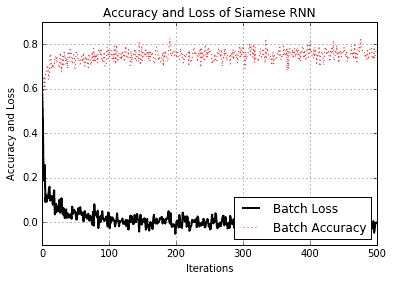我們還可以通過查看訓練期間的損失和準確率來了解模型的執行情況：  圖 9：訓練期間 Siamese RNN 相似性模型的準確率和損失 請注意，我們沒有為此練習指定測試集。這是因為我們如何生成數據。我們創建了一個批量函數，每次調用它時都會創建新的批量數據，因此模型始終可以看到新數據。因此，我們可以使用批量損失和精度作為測試損失和準確率的替代項。但是，對于一組有限的實際數據，情況永遠不會如此，因為我們總是需要訓練和測試集來判斷模型的表現。