# 七、TensorFlow 2 和神經風格遷移 神經風格遷移是一種使用神經網絡將一幅圖像的藝術風格施加到另一幅圖像的內容上的技術，因此最終得到的是兩種圖像的混合體。 您開始使用的圖像稱為**內容圖像**。 您在內容圖像上加上風格的圖像稱為**風格參考圖像**。 Google 將轉換后的圖像稱為**輸入圖像**，這似乎令人困惑（輸入是從兩個不同來源獲取輸入的意思）； 讓我們將其稱為**混合圖像**。 因此，混合圖像是具有風格參考圖像風格的內容圖像。 神經風格遷移通過定義兩個損失函數來工作-一個描述兩個圖像的內容之間的差異，另一個描述兩個圖像之間的風格差異。 為了開始該過程，用內容圖像初始化混合圖像。 然后，使用反向傳播將內容和內容以及混合圖像的風格之間的差異（也稱為損失或距離）最小化。 這將創建具有風格參考圖像風格和內容圖像內容的新圖像（即混合圖像）。 此過程中涉及一些技術-使用函數式 API，使用預訓練的模型及其特征圖以及使用自定義訓練循環以最小化`loss`函數。 我們將在下面的代碼中滿足所有這些要求。 要充分利用該技術，有兩個先決條件-Gatys 等人在 2015 年發表的[原始論文](https://arxiv.org/abs/1508.06576)雖非必要，但確實可以解釋該技術。 技術非常好，因此非常有必要了解如何通過梯度下降來減少損失。 我們將使用 VGG19 架構中的特征層（已在著名的 ImageNet 數據集上進行了訓練，其中包含 1400 萬張圖像和 1000 個類別）。 我們將檢查的代碼源自 Google 提供的代碼； 它使用了急切的執行程序，我們當然不需要編寫代碼，因為它是 TensorFlow 2 中的默認代碼。該代碼在 GPU 上運行得更快，但在耐心等待的情況下仍可以在 CPU 上合理的時間內進行訓練。 在本章中，我們將介紹以下主題： * 配置導入 * 預處理圖像 * 查看原始圖像 * 使用 VGG19 架構 * 建立模型 * 計算損失 * 執行風格遷移 # 配置導入 要對您自己的圖像使用此實現，您需要將這些圖像保存在下載的存儲庫的`./tmp/nst`目錄中，然后編輯`content_path`和`style_path`路徑，如以下代碼所示。 與往常一樣，我們要做的第一件事是導入（并配置）所需的模塊： ```py import numpy as np from PIL import Image import time import functools import matplotlib.pyplot as plt import matplotlib as mpl # set things up for images display mpl.rcParams['figure.figsize'] = (10,10) mpl.rcParams['axes.grid'] = False ``` 您可能需要`pip install pillow`，這是 PIL 的分支。 接下來是 TensorFlow 模塊： ```py import tensorflow as tf from tensorflow.keras.preprocessing import image as kp_image from tensorflow.keras import models from tensorflow.keras import losses from tensorflow.keras import layers from tensorflow.keras import backend as K from tensorflow.keras import optimizers ``` 這是我們最初將使用的兩個圖像： ```py content_path = './tmp/nst/elephant.jpg'#Andrew Shiva / Wikipedia / CC BY-SA 4.0 style_path = './tmp/nst/zebra.jpg' # zebra:Yathin S Krishnappa, https://creativecommons.org/licenses/by-sa/4.0/deed.en ``` # 預處理圖像 下一個函數只需稍作預處理即可加載圖像。 `Image.open()`是所謂的惰性操作。 該函數找到文件并將其打開以進行讀取，但是實際上直到從您嘗試對其進行處理或加載數據以來，才從文件中讀取圖像數據。 下一組三行會調整圖像的大小，以便任一方向的最大尺寸為 512（`max_dimension`）像素。 例如，如果圖像為`1,024 x 768`，則`scale`將為 0.5（`512 / 1,024`），并且這將應用于圖像的兩個尺寸，從而將圖像大小調整為`512 x 384`。`Image.ANTIALIAS`參數保留最佳圖像質量。 接下來，使用`img_to_array()`調用（`tensorflow.keras.preprocessing`的方法）將 PIL 圖像轉換為 NumPy 數組。 最后，為了與以后的使用兼容，圖像需要沿零軸的批次尺寸（由于圖像是彩色的，因此共給出了四個尺寸）。 這可以通過調用`np.expand_dims()`實現： ```py def load_image(path_to_image): max_dimension = 512 image = Image.open(path_to_image) longest_side = max(image.size) scale = max_dimension/longest_side image = image.resize((round(image.size[0]*scale), round(image.size[1]*scale)), Image.ANTIALIAS) image = kp_image.img_to_array(image) # keras preprocessing # Broadcast the image array so that it has a batch dimension on axis 0 image = np.expand_dims(image, axis=0) return image ``` 下一個函數顯示已由`load_image()`預處理過的圖像。 由于我們不需要額外的尺寸來顯示，因此可以通過調用`np.squeeze()`將其刪除。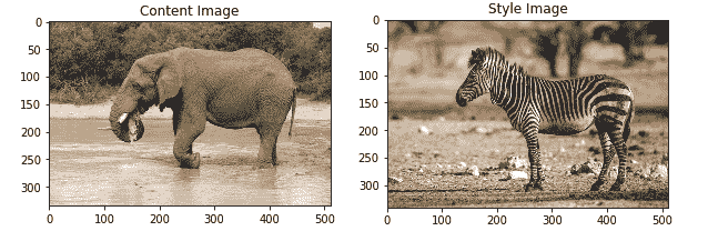 之后，根據對`plt.imshow()`的調用（后面帶有可選標題）的要求，將圖像數據中的值轉換為無符號的 8 位整數： ```py def show_image(image, title=None): # Remove the batch dimension from the image image1 = np.squeeze(image, axis=0) # Normalize the image for display image1 = image1.astype('uint8') plt.imshow(image1) if title is not None: plt.title(title) plt.imshow(image1) ``` # 查看原始圖像 接下來，我們使用對前面兩個函數的調用來顯示內容和風格圖像，請記住圖像像素必須是無符號 8 位整數類型。 `plt.subplot(1,2,1)`函數意味著在位置 1 使用一排兩列的網格； `plt.subplot(1,2,2)`表示在位置 2 使用一排兩列的網格： ```py channel_means = [103.939, 116.779, 123.68] # means of the BGR channels, for VGG processing plt.figure(figsize=(10,10)) content_image = load_image(content_path).astype('uint8') style_image = load_image(style_path).astype('uint8') plt.subplot(1, 2, 1) show_image(content_image, 'Content Image') plt.subplot(1, 2, 2) show_image(style_image, 'Style Image') plt.show() ``` 輸出顯示在以下屏幕截圖中：  接下來是加載圖像的函數。 正如我們將要提到的那樣，在經過訓練的`vgg19`模型中，我們需要相應地預處理圖像數據。 `tf.keras`模塊為我們提供了執行此操作的方法。 這里的預處理將我們的 RGB 彩色圖像翻轉為 BGR： ```py def load_and_process_image(path_to_image): image = load_image(path_to_image) image = tf.keras.applications.vgg19.preprocess_input(image) return image ``` 為了顯示我們的圖像，我們需要一個函數來獲取用`load_and_process_image`處理的數據，并將圖像數據返回到其原始狀態。 這必須手動完成。 首先，我們檢查圖像的尺寸是否正確，如果不是 3 或 4，則會引發錯誤。 預處理從每個通道中減去其平均值，因此通道的平均值為零。 減去的值來自 ImageNet 分析，其中 BGR 通道的均值分別為`103.939`，`116.779`和`123.68`。 因此，接下來，我們將這些值添加回 BGR（彩色）通道以恢復原始值，然后將 BGR 序列翻轉回 RGB。 最后，對于此函數，我們需要確保我們的值是無符號的 8 位整數，其值在 0 到 255 之間； 這可以通過`np.clip()`函數實現： ```py def deprocess_image(processed_image): im = processed_image.copy() if len(im.shape) == 4: im = np.squeeze(im, 0) assert len(im.shape) == 3, ("Input to deprocess image must be an image of " "dimension [1, height, width, channel] or [height, width, channel]") if len(im.shape) != 3: raise ValueError("Invalid input to deprocessing image") # the inverse of the preprocessing step im[:, :, 0] += channel_means[0] # these are the means subtracted by the preprocessing step im[:, :, 1] += channel_means[1] im[:, :, 2] += channel_means[2] im= im[:, :, ::-1] # channel last im = np.clip(im, 0, 255).astype('uint8') return im ``` # 使用 VGG19 架構 了解下一個代碼片段的最好方法是查看 VGG19 架構。 [這是一個好地方](https://github.com/fchollet/deep-learning-models/blob/master/vgg19.py)（大約位于頁面的一半）。 在這里，您將看到 VGG19 是一個相當簡單的體系結構，由卷積層的塊組成，每個塊的末尾都有一個最大池化層。 對于內容層，我們使用`block5`中的第二個卷積層。 之所以使用這個最高的塊，是因為較早的塊具有更能代表單個像素的特征圖。 網絡中的高層會根據對象及其在輸入圖像中的排列來捕獲高級內容，[但不會限制重建的實際精確像素值](https://arxiv.org/abs/1508.06576)。 對于風格層，我們將在每個層塊中使用第一個卷積層，即`block1_conv1`到`block5_conv5`。 然后保存內容和風格層的長度，以供以后使用： ```py # The feature maps are obtained from this content layer content_layers = ['block5_conv2'] # Style layers we need style_layers = ['block1_conv1', 'block2_conv1', 'block3_conv1', 'block4_conv1', 'block5_conv1' ] number_of_content_layers = len(content_layers) number_of_style_layers = len(style_layers) ``` # 建立模型 現在，接下來是一系列函數，這些函數最終導致執行風格遷移（`run_style_transfer()`）的主要函數。 此序列中的第一個函數`get_model()`創建我們將要使用的模型。 它首先加載訓練后的`vgg_model`（已在`ImageNet`上進行訓練），而沒有其分類層（`include_top=False`）。 接下來，它凍結加載的模型（`vgg_model.trainable = False`）。 然后，使用列表推導獲取風格和內容層的輸出值，該列表推導遍歷我們在上一節中指定的層的名稱。 然后將這些輸出值與 VGG 輸入一起使用，以創建可以訪問 VGG 層的新模型，即`get_model()`返回 Keras 模型，該模型輸出已訓練的 VGG19 模型的風格和內容中間層。 不必使用頂層，因為這是 VGG19 中的最終分類層，我們將不再使用。 我們將創建一個輸出圖像，以使輸出和相應特征層上的輸入/風格之間的距離（差異）最小化： ```py def get_model(): vgg_model = tf.keras.applications.vgg19.VGG19(include_top=False, weights='imagenet') vgg_model.trainable = False # Acquire the output layers corresponding to the style layers and the content layers style_outputs = [vgg_model.get_layer(name).output for name in style_layers] content_outputs = [vgg_model.get_layer(name).output for name in content_layers] model_outputs = style_outputs + content_outputs # Build model return models.Model(vgg_model.input, model_outputs) ``` # 計算損失 現在，我們需要兩個圖像的內容和風格之間的損失。 我們將使用均方損失如下。 請注意，`image1 - image2`中的減法是兩個圖像數組之間逐元素的。 此減法有效，因為圖像已在`load_image`中調整為相同大小： ```py def rms_loss(image1,image2): loss = tf.reduce_mean(input_tensor=tf.square(image1 - image2)) return loss ``` 接下來，我們定義`content_loss`函數。 這只是函數簽名中`content`和`target`之間的均方差： ```py def content_loss(content, target): return rms_loss(content, target) ``` 風格損失是根據稱為 **Gram 矩陣**的數量定義的。 Gram 矩陣（也稱為度量）是風格矩陣及其自身的轉置的點積。 因為這意味著圖像矩陣的每一列都與每一行相乘，所以我們可以認為原始表示中包含的空間信息已經*分配*。 結果是有關圖像的非本地化信息，例如紋理，形狀和權重，即其風格。 產生`gram_matrix`的代碼如下： ```py def gram_matrix(input_tensor): channels = int(input_tensor.shape[-1]) # channels is last dimension tensor = tf.reshape(input_tensor, [-1, channels]) # Make the image channels first number_of_channels = tf.shape(input=tensor)[0] # number of channels gram = tf.matmul(tensor, tensor, transpose_a=True) # produce tensorT*tensor return gram / tf.cast(number_of_channels, tf.float32) # scaled by the number of channels. ``` 因此，風格損失（其中`gram_target`將是混合圖像上風格激活的 Gram 矩陣）如下： ```py def style_loss(style, gram_target): gram_style = gram_matrix(style) return rms_loss(gram_style, gram_target) ``` 接下來，我們通過獲取`content_image`和`style_image`并將它們饋入模型來找到`content_features`和`style_features`表示形式。 此代碼分為兩個塊，一個用于`content_features`，另一個用于`style_features`。 對于內容塊，我們加載圖像，在其上調用我們的模型，最后，提取先前分配的特征層。 `style_features`的代碼是相同的，除了我們首先加載風格圖像： ```py def get_feature_representations(model, content_path, style_path): #Function to compute content and style feature representations. content_image = load_and_process_image(content_path) content_outputs = model(content_image) #content_features = [content_layer[0] for content_layer in content_outputs[:number_of_content_layers]] content_features = [content_layer[0] for content_layer in content_outputs[number_of_style_layers:]] style_image = load_and_process_image(style_path) style_outputs = model(style_image) style_features = [style_layer[0] for style_layer in style_outputs[:number_of_style_layers]] return style_features, content_features ``` 接下來，我們需要計算總損失。 查看該方法的簽名，我們可以看到，首先，我們傳入模型（可以訪問 VGG19 的中間層）。 接下來，進入`loss_weights`，它們是每個損失函數（`content_weight`，`style_weight`和總變化權重）的每個貢獻的權重。 然后，我們有了初始圖像，即我們正在通過優化過程更新的圖像。 接下來是`gram_style_features`和`content_features`，分別對應于我們正在使用的風格層和內容層。 首先從方法簽名中復制風格和`content_weight`。 然后，在我們的初始圖像上調用模型。 我們的模型可以直接調用，因為我們使用的是急切執行，如我們所見，這是 TensorFlow 2 中的默認執行。此調用返回所有模型輸出值。 然后，我們有兩個類似的塊，一個塊用于內容，一個塊用于風格。 對于第一個（內容）塊，獲取我們所需層中的內容和風格表示。 接下來，我們累積來自所有內容損失層的內容損失，其中每一層的貢獻均被加權。 第二個塊與第一個塊相似，不同之處在于，這里我們累積來自所有風格損失層的風格損失，其中每個損失層的每個貢獻均被平均加權。 最后，該函數返回總損失，風格損失和內容損失，如以下代碼所示： ```py def compute_total_loss(model, loss_weights, init_image, gram_style_features, content_features): style_weight, content_weight = loss_weights model_outputs = model(init_image) content_score = 0 content_output_features = model_outputs[number_of_style_layers:] weight_per_content_layer = 1.0 / float(number_of_content_layers) for target_content, comb_content in zip(content_features, content_output_features): content_score += weight_per_content_layer*content_loss(comb_content[0], target_content) content_score *= content_weight style_score = 0 style_output_features = model_outputs[:number_of_style_layers] weight_per_style_layer = 1.0 / float(number_of_style_layers) for target_style, comb_style in zip(gram_style_features, style_output_features): style_score += weight_per_style_layer *style_loss(comb_style[0], target_style) style_score ***= style_weight total_loss = style_score + content_score return total_loss, style_score, content_score ``` 接下來，我們有一個計算梯度的函數： ```py def compute_grads(config): with tf.GradientTape() as tape: all_loss = compute_total_loss(**config) # Compute gradients wrt input image total_loss = all_loss[0] return tape.gradient(total_loss, config['init_image']), all_loss import IPython.display ``` # 執行風格遷移 執行`style_transfer`的函數很長，因此我們將分節介紹。 其簽名如下： ```py def run_style_transfer(content_path, style_path, number_of_iterations=1000, content_weight=1e3, style_weight=1e-2): ``` 由于我們實際上不想訓練模型中的任何層，因此只需使用如前所述的層的輸出值即可。 我們相應地設置其可訓練屬性： ```py model = get_model() for layer in model.layers: layer.trainable = False ``` 接下來，我們使用先前定義的函數從模型的各層獲得`style_features`和`content_features`表示形式： ```py style_features, content_features = get_feature_representations(model, content_path, style_path) ``` `gram_style_features`使用`style_features`上的循環，如下所示： ```py gram_style_features = [gram_matrix(style_feature) for style_feature in style_features] ``` 接下來，我們通過加載內容圖像并將其轉換為張量，來初始化將成為算法輸出的圖像，即混合圖像（也稱為 **Pastiche 圖像**）： ```py initial_image = load_and_process_image(content_path) initial_image = tf.Variable(initial_image, dtype=tf.float32) ``` 下一行定義所需的`AdamOptimizer`函數： ```py optimizer = tf.compat.v1.train.AdamOptimizer(learning_rate=5, beta1=0.99, epsilon=1e-1) ``` 我們將繼續保存`best_image`和`best_loss`，因此請初始化變量以存儲它們： ```py best_loss, best_image = float('inf'), None ``` 接下來，我們設置將被傳遞到`compute_grads()`函數的配置值字典： ```py loss_weights = (style_weight, content_weight) config = { 'model': model, 'loss_weights': loss_weights, 'init_image': initial_image, 'gram_style_features': gram_style_features, 'content_features': content_features } ``` 這是顯示常量： ```py number_rows = 2 number_cols = 5 display_interval = number_of_iterations/(number_rows*number_cols) ``` 接下來，我們計算圖像邊界，如下所示： ```py norm_means = np.array(channel_means) minimum_vals = -norm_means maximum_vals = 255 - norm_means ``` 此列表將存儲混合圖像： ```py images = [] ``` 接下來，我們開始主圖像處理循環，如下所示： ```py for i in range(number_of_iterations): ``` 因此，接下來我們計算梯度，計算損失，調用優化器以應用梯度，并將圖像裁剪到我們先前計算的邊界： ```py grads, all_loss = compute_grads(config) loss, style_score, content_score = all_loss optimizer.apply_gradients([(grads, initial_image)]) clipped_image = tf.clip_by_value(initial_image, minimum_vals, maximum_vals) initial_image.assign(clipped_image) ``` 我們將繼續保存`best_loss`和`best_image`，因此下一步： ```py if loss < best_loss: # Update best loss and best image from total loss. 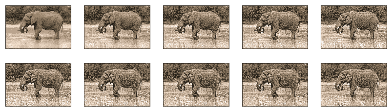best_loss = loss best_image = deprocess_image(initial_image.numpy() ``` 然后，我們有條件地保存混合圖像（總共 10 張圖像），并將其與訓練指標一起顯示： ```py if i % display_interval== 0: # Use the .numpy() method to get the numpy image array, needs eager execution plot_image = initial_image.numpy() plot_image = deprocess_image(plot_image) images.append(plot_image) IPython.display.clear_output(wait=True) IPython.display.display_png(Image.fromarray(plot_image)) print('Iteration: {}'.format(i)) print('Total loss: {:.4e}, ' 'style loss: {:.4e}, ' 'content loss: {:.4e} ' .format(loss, style_score, content_score)) ``` 最后，對于此函數，我們顯示所有`best_image`和`best_loss`： ```py IPython.display.clear_output(wait=True) plt.figure(figsize=(14,4)) for i,image in enumerate(images): plt.subplot(number_rows,number_cols,i+1) plt.imshow(image) plt.xticks([]) plt.yticks([]) return best_image, best_loss ``` 接下來，我們調用前面的函數來獲取`best_image`和`best_loss`（還將顯示 10 張圖像）：  的代碼如下： ```py best_image, best_loss = run_style_transfer(content_path, style_path, number_of_iterations=100) Image.fromarray(best_image) ``` 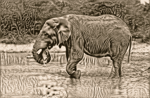以下是`best_image`的顯示：  # 最終展示 最后，我們有一個函數，它與`best_image`一起顯示內容和風格圖像： ```py def show_results(best_image, content_path, style_path, show_large_final=True): plt.figure(figsize=(10, 5)) content = load_image(content_path) style = load_image(style_path) plt.subplot(1, 2, 1) show_image(content, 'Content Image') plt.subplot(1, 2, 2) show_image(style, 'Style Image') if show_large_final: plt.figure(figsize=(10, 10)) plt.imshow(best_image) plt.title('Output Image') plt.show() ``` 接下來是對該函數的調用，如下所示： ```py show_results(best_image, content_path, style_path) ``` # 總結 到此結束我們對神經風格遷移的研究。 我們看到了如何拍攝內容圖像和風格圖像并生成混合圖像。 我們使用訓練有素的 VGG19 模型中的層來完成此任務。 在下一章中，我們將研究循環神經網絡。 這些網絡可以處理順序的輸入值，并且輸入值和輸出值中的一個或兩個具有可變長度。