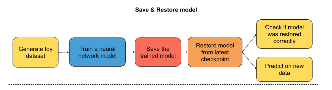
# 三、如何保存和恢復訓練模型 滾動瀏覽`reddit.com/r/learnmachinelearning`的帖子后，我意識到機器學習項目的主要瓶頸，出現于數據輸入流水線和模型的最后階段，你必須保存模型和 對新數據做出預測。 所以我認為制作一個簡單直接的教程，向你展示如何保存和恢復使用 Tensorflow Eager 構建的模型會很有用。 教程的流程圖  ## 導入有用的庫 ```py # 導入 TensorFlow 和 TensorFlow Eager import tensorflow as tf import tensorflow.contrib.eager as tfe # 導入函數來生成玩具分類問題 from sklearn.datasets import make_moons # 開啟 Eager 模式。一旦開啟不能撤銷！只執行一次。 tfe.enable_eager_execution() ``` ## 第一部分：為二分類構建簡單的神經網絡 ```py class simple_nn(tf.keras.Model): def __init__(self): super(simple_nn, self).__init__() """ 在這里定義正向傳播期間 使用的神經網絡層 """ # 隱層 self.dense_layer = tf.layers.Dense(10, activation=tf.nn.relu) # 輸出層，無激活 self.output_layer = tf.layers.Dense(2, activation=None) def predict(self, input_data): """ 在神經網絡上執行正向傳播 Args: input_data: 2D tensor of shape (n_samples, n_features). Returns: logits: unnormalized predictions. """ hidden_activations = self.dense_layer(input_data) logits = self.output_layer(hidden_activations) return logits def loss_fn(self, input_data, target): """ 定義訓練期間使用的損失函數 """ logits = self.predict(input_data) loss = tf.losses.sparse_softmax_cross_entropy(labels=target, logits=logits) return loss def grads_fn(self, input_data, target): """ 在每個正向步驟中， 動態計算損失值對模型參數的梯度 """ with tfe.GradientTape() as tape: loss = self.loss_fn(input_data, target) return tape.gradient(loss, self.variables) def fit(self, input_data, target, optimizer, num_epochs=500, verbose=50): """ 用于訓練模型的函數， 使用所選的優化器，執行所需數量的迭代 """ for i in range(num_epochs): grads = self.grads_fn(input_data, target) optimizer.apply_gradients(zip(grads, self.variables)) if (i==0) | ((i+1)%verbose==0): print('Loss at epoch %d: %f' %(i+1, self.loss_fn(input_data, target).numpy())) ``` ## 第二部分：訓練模型 ```py # 為分類生成玩具數據集 # X 是 n_samples x n_features 的矩陣，表示輸入特征 # y 是 長度為 n_samples 的向量，表示我們的標簽 X, y = make_moons(n_samples=100, noise=0.1, random_state=2018) X_train, y_train = tf.constant(X[:80,:]), tf.constant(y[:80]) X_test, y_test = tf.constant(X[80:,:]), tf.constant(y[80:]) optimizer = tf.train.GradientDescentOptimizer(5e-1) model = simple_nn() model.fit(X_train, y_train, optimizer, num_epochs=500, verbose=50) ''' Loss at epoch 1: 0.658276 Loss at epoch 50: 0.302146 Loss at epoch 100: 0.268594 Loss at epoch 150: 0.247425 Loss at epoch 200: 0.229143 Loss at epoch 250: 0.197839 Loss at epoch 300: 0.143365 Loss at epoch 350: 0.098039 Loss at epoch 400: 0.070781 Loss at epoch 450: 0.053753 Loss at epoch 500: 0.042401 ''' ``` ## 第三部分：保存訓練模型 ```py # 指定檢查點目錄 checkpoint_directory = 'models_checkpoints/SimpleNN/' # 創建模型檢查點 checkpoint = tfe.Checkpoint(optimizer=optimizer, model=model, optimizer_step=tf.train.get_or_create_global_step()) # 保存訓練模型 checkpoint.save(file_prefix=checkpoint_directory) # 'models_checkpoints/SimpleNN/-1' ``` ## 第四部分：恢復訓練模型 ```py # 重新初始化模型實例 model = simple_nn() optimizer = tf.train.GradientDescentOptimizer(5e-1) # 指定檢查點目錄 checkpoint_directory = 'models_checkpoints/SimpleNN/' # 創建模型檢查點 checkpoint = tfe.Checkpoint(optimizer=optimizer, model=model, optimizer_step=tf.train.get_or_create_global_step()) # 從最近的檢查點恢復模型 checkpoint.restore(tf.train.latest_checkpoint(checkpoint_directory)) # <tensorflow.contrib.eager.python.checkpointable_utils.CheckpointLoadStatus at 0x7fcfd47d2048> ``` ## 第五部分：檢查模型是否正確恢復 ```py model.fit(X_train, y_train, optimizer, num_epochs=1) # Loss at epoch 1: 0.042220 ``` 損失似乎與我們在之前訓練的最后一個迭代中獲得的損失一致！ ## 第六部分：對新數據做預測 ```py logits_test = model.predict(X_test) print(logits_test) ''' tf.Tensor( [[ 1.54352813 -0.83117302] [-1.60523365 2.82397487] [ 2.87589525 -1.36463485] [-1.39461001 2.62404279] [ 0.82305161 -0.55651397] [ 3.53674391 -2.55593046] [-2.97344627 3.46589599] [-1.69372442 2.95660466] [-1.43226137 2.65357974] [ 3.11479995 -1.31765645] [-0.65841567 1.60468631] [-2.27454367 3.60553595] [-1.50170912 2.74410115] [ 0.76261479 -0.44574208] [ 2.34516959 -1.6859307 ] [ 1.92181942 -1.63766352] [ 4.06047684 -3.03988941] [ 1.00252324 -0.78900484] [ 2.79802993 -2.2139734 ] [-1.43933035 2.68037059]], shape=(20, 2), dtype=float64) ''' ```