# 六、循環神經網絡 在本章中，我們將介紹一些涵蓋以下主題的秘籍： * 神經機器翻譯-訓練 seq2seq RNN * 神經機器翻譯-推理 seq2seq RNN * 您只需要關注-seq2seq RNN 的另一個示例 * 通過 RNN 學習寫作莎士比亞 * 學習使用 RNN 預測未來的比特幣價值 * 多對一和多對多 RNN 示例 # 介紹 在本章中，我們將討論**循環神經網絡**（**RNN**）如何在保持順序順序重要的領域中用于深度學習。 我們的注意力將主要集中在文本分析和**自然語言處理**（**NLP**）上，但我們還將看到用于預測比特幣價值的序列示例。 通過采用基于時間序列的模型，可以描述許多實時情況。 例如，如果您考慮編寫文檔，則單詞的順序很重要，而當前單詞肯定取決于先前的單詞。 如果我們仍然專注于文本編寫，很明顯單詞中的下一個字符取決于前一個字符（例如`quick brown`字符的下一個字母很有可能將會是字母`fox`），如下圖所示。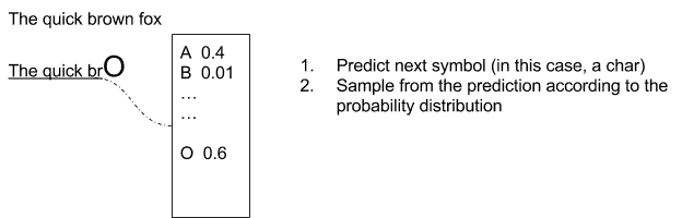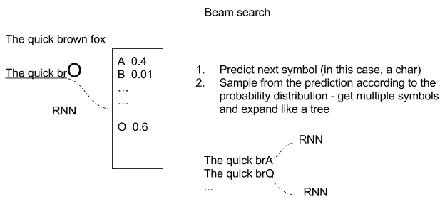 關鍵思想是在給定當前上下文的情況下生成下一個字符的分布，然后從該分布中采樣以生成下一個候選字符：  用`The quick brown fox`句子進行預測的例子 一個簡單的變體是存儲多個預測，因此創建一棵可能的擴展樹，如下圖所示：  `The quick brown fox`句子的預測樹的示例 但是，基于序列的模型可以在大量其他域中使用。 在音樂中，樂曲中的下一個音符肯定取決于前一個音符，而在視頻中，電影中的下一個幀必定與前一幀有關。 此外，在某些情況下，當前的視頻幀，單詞，字符或音符不僅取決于前一個，而且還取決于后一個。 可以使用 RNN 描述基于時間序列的模型，其中對于給定輸入`X[i]`，時間為`i`，產生輸出`Y[i]`，將時間`[0，i-1]`的以前狀態的記憶反饋到網絡。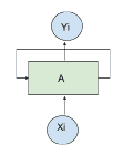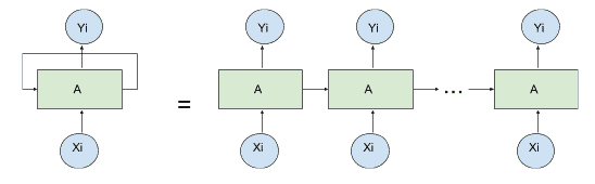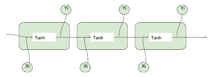 反饋先前狀態的想法由循環循環描述，如下圖所示： ；  反饋示例 循環關系可以方便地通過*展開*網絡來表示，如下圖所示：  展開循環單元的例子 最簡單的 RNN 單元由簡單的 *tanh* 函數（雙曲正切函數）組成，如下圖所示：   個簡單的 tanh 單元的例子 # 梯度消失和爆炸 訓練 RNN 十分困難，因為存在兩個穩定性問題。 由于反饋回路的緣故，梯度可能會迅速發散到無窮大，或者它可能會迅速發散到 0。在兩種情況下，如下圖所示，網絡將停止學習任何有用的東西。 可以使用基于**梯度修剪**的相對簡單的解決方案來解決梯度爆炸的問題。 梯度消失的問題更難解決，它涉及更復雜的 RNN 基本單元的定義，例如**長短期記憶**（**LSTM**）或**門控循環單元**（**GRU**）。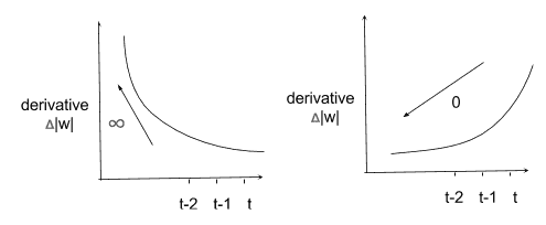 讓我們首先討論梯度爆炸和梯度裁剪：  梯度示例 **梯度裁剪**包括對梯度施加最大值，以使其無法無限增長。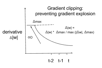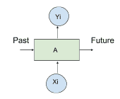 下圖所示的簡單解決方案為**梯度爆炸問題提供了簡單的解決方案**：  梯度裁剪的例子 解決梯度消失的問題需要一種更復雜的內存模型，該模型可以選擇性地忘記先前的狀態，只記住真正重要的狀態。 考慮下圖，輸入以`[0,1]`中的概率`p`寫入存儲器`M`中，并乘以加權輸入。 以類似的方式，以`[0,1]`中的概率`p`讀取輸出，將其乘以加權輸出。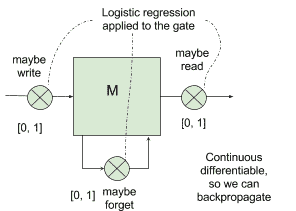 還有一種可能性用來決定要記住或忘記的事情：  存儲單元的一個例子 # 長短期記憶（LSTM） LSTM 網絡可以控制何時讓輸入進入神經元，何時記住在上一個時間步中學到的內容以及何時讓輸出傳遞到下一個時間戳。 所有這些決定都是自調整的，并且僅基于輸入。 乍一看，LSTM 看起來很難理解，但事實并非如此。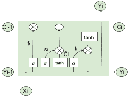 讓我們用下圖來說明它是如何工作的：  LSTM 單元的一個例子 首先，我們需要一個邏輯函數σ（請參見第 2 章，“回歸”）來計算介于 0 和 1 之間的值，并控制哪些信息流過 *LSTM 門*。 請記住，邏輯函數是可微的，因此允許反向傳播。 然后，我們需要一個運算符`?`，它采用兩個相同維的矩陣并生成另一個矩陣，其中每個元素`ij`是原始兩個矩陣的元素`ij`的乘積。 同樣，我們需要一個運算符`⊕`，它采用兩個相同維度的矩陣并生成另一個矩陣，其中每個元素`ij`是原始兩個矩陣的元素`ij`之和。 使用這些基本塊，我們考慮時間`i`處的輸入`X[i]`，并將其與上一步中的輸出`Y[i-1]`并置。 方程`f[t] = σ(W[f] · [y[i-1], x[t]] + b[f])`實現了控制激活門`?`的邏輯回歸，并用于確定應從*先前*候選值`C[i-1]`獲取多少信息。 傳遞給下一個候選值`C[i]`（此處`W[f]`和`b[f]`矩陣和用于邏輯回歸的偏差）。如果 Sigmoid 輸出為 1，則表示*不要忘記*先前的單元格狀態`C[i-1]`；如果輸出 0， 這將意味著*忘記*先前的單元狀態`C[i-1]`。`(0, 1)`中的任何數字都將表示要傳遞的信息量。 然后我們有兩個方程：`s[i] = σ(W[s] · [Y[i-1], x[i]] + b[s])`，用于通過`?`控制由當前單元產生的多少信息（`?[i] = tanh(W [C] · [Y[i-1]， X[i] + b[c])`）應該通過`⊕`運算符添加到下一個候選值`C[i]`中，根據上圖中表示的方案。 為了實現與運算符`⊕`和`?`所討論的內容，我們需要另一個方程，其中進行實際的加法`+`和乘法`*`：`C[i] = f[t] * C[i-1] + s[i] * ?[i]` 最后，我們需要確定當前單元格的哪一部分應發送到`Y[i]`輸出。 這很簡單：我們再進行一次邏輯回歸方程，然后通過`?`運算來控制應使用哪一部分候選值輸出。 在這里，有一點值得關注，使用 *tanh* 函數將輸出壓縮為`[-1, 1]`。 最新的步驟由以下公式描述：  現在，我了解到這看起來像很多數學運算，但有兩個好消息。 首先，如果您了解我們想要實現的目標，那么數學部分并不是那么困難。 其次，您可以將 LSTM 單元用作標準 RNN 單元的黑盒替代，并立即獲得解決梯度消失問題的好處。 因此，您實際上不需要了解所有數學知識。 您只需從庫中獲取 TensorFlow LSTM 實現并使用它即可。 # 門控循環單元（GRU）和窺孔 LSTM 近年來提出了許多 LSTM 單元的變體。 其中兩個真的很受歡迎。 窺孔 LSTM 允許柵極層查看單元狀態，如下圖虛線所示，而**門控循環單元**（**GRU**）將隱藏狀態和單元狀態和合并為一個單一的信息渠道。 同樣，GRU 和 Peephole LSTM 都可以用作標準 RNN 單元的黑盒插件，而無需了解基礎數學。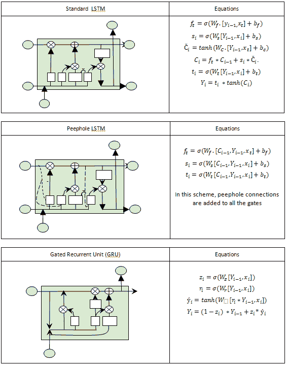 這兩個單元都可用于解決梯度消失的問題，并可用于構建深度神經網絡：  標準 LSTM，PeepHole LSTM 和 GRU 的示例 # 向量序列的運算 使 RNN 真正強大的是能夠對向量序列進行操作的能力，其中 RNN 的輸入和/或 RNN 的輸出都可以是序列。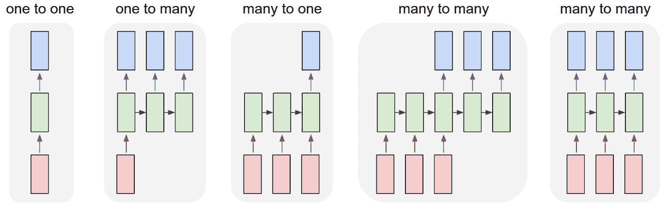 下圖很好地表示了這一點，其中最左邊的示例是傳統的（非循環）網絡，其后是帶有輸出序列的 RNN，然后是帶有輸入序列的 RNN，再是帶有序列的 RNN 在不同步序列的輸入和輸出中，然后是在序列同步的輸入和輸出中具有序列的 RNN：  [RNN 序列的一個例子](http://karpathy.github.io/2015/05/21/rnn-effectiveness/) 機器翻譯是輸入和輸出中不同步序列的一個示例：網絡將輸入文本作為序列讀取，在讀取全文之后，*會輸出目標語言*。 視頻分類是輸入和輸出中同步序列的示例：視頻輸入是幀序列，并且對于每個幀，輸出中都提供了分類標簽。 如果您想了解有關 RNN 有趣應用的更多信息，則必須閱讀 Andrej Karpathy [發布的博客](http://karpathy.github.io/2015/05/21/rnn-effectiveness/)。 他訓練了網絡，以莎士比亞的風格撰寫論文（用 Karpathy 的話說：*幾乎*不能從實際的莎士比亞中識別出這些樣本），撰寫有關虛構主題的現實 Wikipedia 文章，撰寫關于愚蠢和不現實問題的現實定理證明（用 Karpathy 的話：*更多的幻覺代數幾何*），并寫出現實的 Linux 代碼片段（用 Karpathy 的話：*他首先建模逐個字符地列舉 GNU 許可證，其中包括一些示例，然后生成一些宏，然后深入研究代碼*）。 以下示例摘自[這個頁面](http://karpathy.github.io/2015/05/21/rnn-effectiveness/)：  用 RNN 生成的文本示例 # 神經機器翻譯 -- 訓練 seq2seq RNN 序列到序列（seq2seq）是 RNN 的一種特殊類型，已成功應用于神經機器翻譯，文本摘要和語音識別中。 在本秘籍中，我們將討論如何實現神經機器翻譯，其結果與 [Google 神經機器翻譯系統](https://research.googleblog.com/2016/09/a-neural-network-for-machine.html)。 關鍵思想是輸入整個文本序列，理解整個含義，然后將翻譯輸出為另一個序列。 讀取整個序列的想法與以前的架構大不相同，在先前的架構中，將一組固定的單詞從一種源語言翻譯成目標語言。 本節的靈感來自 [Minh-Thang Luong](https://github.com/lmthang/thesis/blob/master/thesis.pdf) 的 2016 年博士學位論文《神經機器翻譯》。 第一個關鍵概念是編碼器-解碼器架構的存在，其中編碼器將源句子轉換為代表含義的向量。 然后，此向量通過解碼器以產生翻譯。 編碼器和解碼器都是 RNN，它們可以捕獲語言中的長期依賴關系，例如性別協議和語法結構，而無需先驗地了解它們，并且不需要跨語言進行 1：1 映射。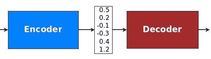 這是一種強大的功能，可實現非常流暢的翻譯：  [編解碼器的示例](https://github.com/lmthang/thesis/blob/master/thesis.pdf) 讓我們看一個 RNN 的示例，該語句將`She loves cute cats`翻譯成`Elle Aime les chat Mignons`。 有兩種 RNN：一種充當編碼器，另一種充當解碼器。 源句`She loves cute cats`后跟一個分隔符-目標句是`Elle aime les chats mignons`。 這兩個連接的句子在輸入中提供給編碼器進行訓練，并且解碼器將生成目標目標。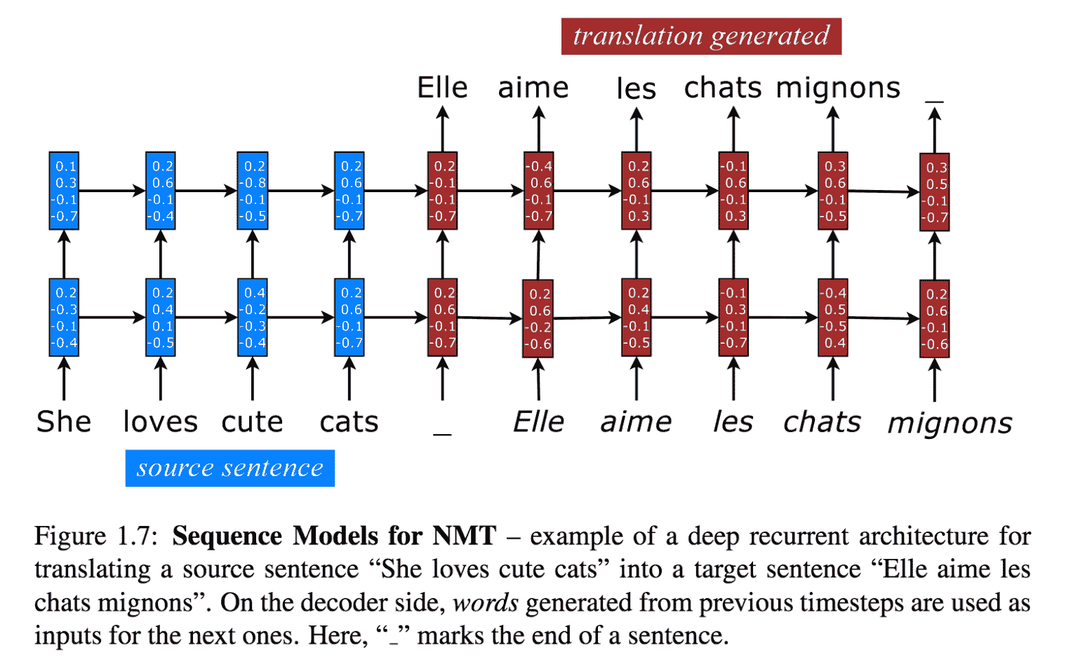 當然，我們需要像這樣的多個示例來獲得良好的訓練：  [NMT 序列模型的示例](https://github.com/lmthang/thesis/blob/master/thesis.pdf) 現在，我們可以擁有許多 RNN 變體。 讓我們看看其中的一些： * RNN 可以是單向或雙向的。 后者將捕捉雙方的長期關系。 * RNN 可以具有多個隱藏層。 選擇是關于優化的問題：一方面，更深的網絡可以學到更多；另一方面，更深的網絡可以學到更多。 另一方面，可能需要很長的時間來訓練并且可能會過頭。 * RNN 可以具有一個嵌入層，該層將單詞映射到一個嵌入空間中，在該空間中相似的單詞恰好被映射得非常近。 * RNNs 可以使用簡單的或者循環的單元，或 LSTM，或窺視孔 LSTM，或越冬。 仍然參考博士學位論文[《神經機器翻譯》](https://github.com/lmthang/thesis/blob/master/thesis.pdf)，我們可以使用嵌入層來將輸入語句放入嵌入空間。 然后，有兩個 RNN *粘在一起*——源語言的編碼器和目標語言的解碼器。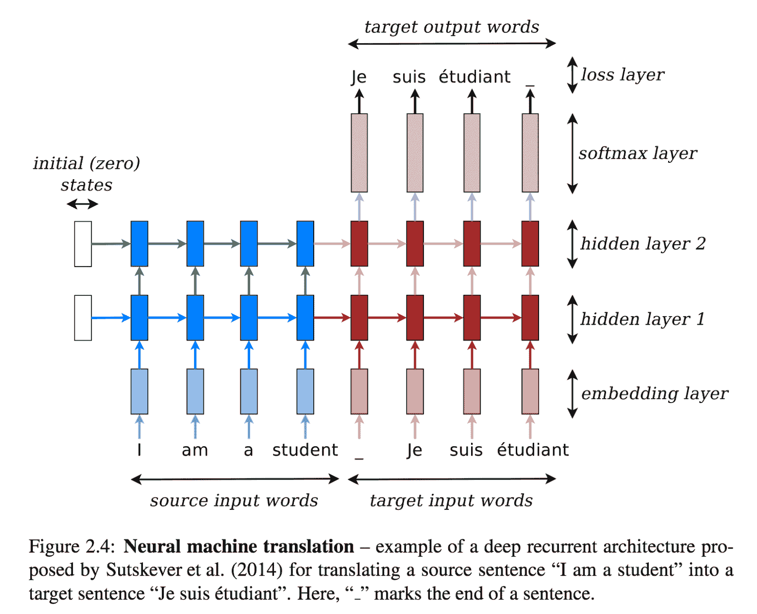 如您所見，存在多個隱藏層，并且有兩個流程：前饋垂直方向連接這些隱藏層，水平方向是將知識從上一步轉移到下一層的循環部分：  [神經機器翻譯的例子](https://github.com/lmthang/thesis/blob/master/thesis.pdf) 在本秘籍中，我們使用 NMT（神經機器翻譯），這是一個可在 TensorFlow 頂部在線獲得的翻譯演示包。 # 準備 NMT 可在[這個頁面](https://github.com/tensorflow/nmt/)上找到，并且代碼在 GitHub 上。 # 操作步驟 我們按以下步驟進行： 1. 從 GitHub 克隆 NMT： ```py git clone https://github.com/tensorflow/nmt/ ``` 2. 下載訓練數據集。 在這種情況下，我們將使用訓練集將越南語翻譯為英語。 其他數據集可從[這里](https://nlp.stanford.edu/projects/nmt/)獲取其他語言，例如德語和捷克語： ```py nmt/scripts/download_iwslt15.sh /tmp/nmt_data ``` 3. 考慮[這里](https://github.com/tensorflow/nmt/)，我們將定義第一個嵌入層。 嵌入層接受輸入，詞匯量 V 和輸出嵌入空間的所需大小。 詞匯量使得僅考慮 V 中最頻繁的單詞進行嵌入，而所有其他單詞都映射到一個常見的*未知*項。 在我們的例子中，輸入是主要時間的，這意味著最大時間是[第一個輸入參數](https://www.tensorflow.org/api_docs/python/tf/nn/dynamic_rnn)： ```py # Embedding embedding_encoder = variable_scope.get_variable( "embedding_encoder", [src_vocab_size, embedding_size], ...) # Look up embedding: # encoder_inputs: [max_time, batch_size] # encoder_emb_inp: [max_time, batch_size, embedding_size] encoder_emb_inp = embedding_ops.embedding_lookup( embedding_encoder, encoder_inputs) ``` 4. 仍然參考[這里](https://github.com/tensorflow/nmt/)，我們定義了一個簡單的編碼器，它使用`tf.nn.rnn_cell.BasicLSTMCell(num_units)`作為基本 RNN 單元。 這非常簡單，但是要注意，給定基本的 RNN 單元，我們使用[`tf.nn.dynamic_rnn`](https://www.tensorflow.org/api_docs/python/tf/nn/dynamic_rnn)創建 RNN： ```py # Build RNN cell encoder_cell = tf.nn.rnn_cell.BasicLSTMCell(num_units) # Run Dynamic RNN # encoder_outpus: [max_time, batch_size, num_units] # encoder_state: [batch_size, num_units] encoder_outputs, encoder_state = tf.nn.dynamic_rnn( encoder_cell, encoder_emb_inp, sequence_length=source_sequence_length, time_major=True) ``` 5. 之后，我們需要定義解碼器。 因此，第一件事是擁有一個帶有`tf.nn.rnn_cell.BasicLSTMCell`的基本 RNN 單元，然后將其用于創建一個基本采樣解碼器`tf.contrib.seq2seq.BasicDecoder`，該基本采樣解碼器將用于與解碼器`tf.contrib.seq2seq.dynamic_decode`進行動態解碼： ```py # Build RNN cell decoder_cell = tf.nn.rnn_cell.BasicLSTMCell(num_units) # Helper helper = tf.contrib.seq2seq.TrainingHelper( decoder_emb_inp, decoder_lengths, time_major=True) # Decoder decoder = tf.contrib.seq2seq.BasicDecoder( decoder_cell, helper, encoder_state, output_layer=projection_layer) # Dynamic decoding outputs, _ = tf.contrib.seq2seq.dynamic_decode(decoder, ...) logits = outputs.rnn_output ``` 6. 網絡的最后一個階段是 softmax 密集階段，用于將頂部隱藏狀態轉換為對率向量： ```py projection_layer = layers_core.Dense( tgt_vocab_size, use_bias=False) ``` 7. 當然，我們需要定義交叉熵函數和訓練階段使用的損失： ```py crossent = tf.nn.sparse_softmax_cross_entropy_with_logits( labels=decoder_outputs, logits=logits) train_loss = (tf.reduce_sum(crossent * target_weights) / batch_size) ``` 8. 下一步是定義反向傳播所需的步驟，并使用適當的優化器（在本例中為 Adam）。 請注意，梯度已被裁剪，Adam 使用預定義的學習率： ```py # Calculate and clip gradients params = tf.trainable_variables() gradients = tf.gradients(train_loss, params) clipped_gradients, _ = tf.clip_by_global_norm( gradients, max_gradient_norm) # Optimization optimizer = tf.train.AdamOptimizer(learning_rate) update_step = optimizer.apply_gradients( zip(clipped_gradients, params)) ``` 9. 現在，我們可以運行代碼并了解不同的執行步驟。 首先，創建訓練圖。 然后，訓練迭代開始。 用于評估的度量標準是**雙語評估研究**（**BLEU**）。 此度量標準是評估已從一種自然語言機器翻譯成另一種自然語言的文本質量的標準。 質量被認為是機器與人工輸出之間的對應關系。 如您所見，該值隨時間增長： ```py python -m nmt.nmt --src=vi --tgt=en --vocab_prefix=/tmp/nmt_data/vocab --train_prefix=/tmp/nmt_data/train --dev_prefix=/tmp/nmt_data/tst2012 --test_prefix=/tmp/nmt_data/tst2013 --out_dir=/tmp/nmt_model --num_train_steps=12000 --steps_per_stats=100 --num_layers=2 --num_units=128 --dropout=0.2 --metrics=bleu # Job id 0 [...] # creating train graph ... num_layers = 2, num_residual_layers=0 cell 0 LSTM, forget_bias=1 DropoutWrapper, dropout=0.2 DeviceWrapper, device=/gpu:0 cell 1 LSTM, forget_bias=1 DropoutWrapper, dropout=0.2 DeviceWrapper, device=/gpu:0 cell 0 LSTM, forget_bias=1 DropoutWrapper, dropout=0.2 DeviceWrapper, device=/gpu:0 cell 1 LSTM, forget_bias=1 DropoutWrapper, dropout=0.2 DeviceWrapper, device=/gpu:0 start_decay_step=0, learning_rate=1, decay_steps 10000,decay_factor 0.98 [...] # Start step 0, lr 1, Thu Sep 21 12:57:18 2017 # Init train iterator, skipping 0 elements global step 100 lr 1 step-time 1.65s wps 3.42K ppl 1931.59 bleu 0.00 global step 200 lr 1 step-time 1.56s wps 3.59K ppl 690.66 bleu 0.00 [...] global step 9100 lr 1 step-time 1.52s wps 3.69K ppl 39.73 bleu 4.89 global step 9200 lr 1 step-time 1.52s wps 3.72K ppl 40.47 bleu 4.89 global step 9300 lr 1 step-time 1.55s wps 3.62K ppl 40.59 bleu 4.89 [...] # External evaluation, global step 9000 decoding to output /tmp/nmt_model/output_dev. done, num sentences 1553, time 17s, Thu Sep 21 17:32:49 2017. bleu dev: 4.9 saving hparams to /tmp/nmt_model/hparams # External evaluation, global step 9000 decoding to output /tmp/nmt_model/output_test. done, num sentences 1268, time 15s, Thu Sep 21 17:33:06 2017. bleu test: 3.9 saving hparams to /tmp/nmt_model/hparams [...] global step 9700 lr 1 step-time 1.52s wps 3.71K ppl 38.01 bleu 4.89 ``` # 工作原理 所有上述代碼已在[這個頁面](https://github.com/tensorflow/nmt/blob/master/nmt/model.py)中定義。 關鍵思想是將兩個 RNN *打包在一起*。 第一個是編碼器，它在嵌入空間中工作，非常緊密地映射相似的單詞。 編碼器*理解*訓練示例的含義，并產生張量作為輸出。 然后只需將編碼器的最后一個隱藏層連接到解碼器的初始層，即可將該張量傳遞給解碼器。 注意力學習是由于我們基于與`labels=decoder_outputs`的交叉熵的損失函數而發生的。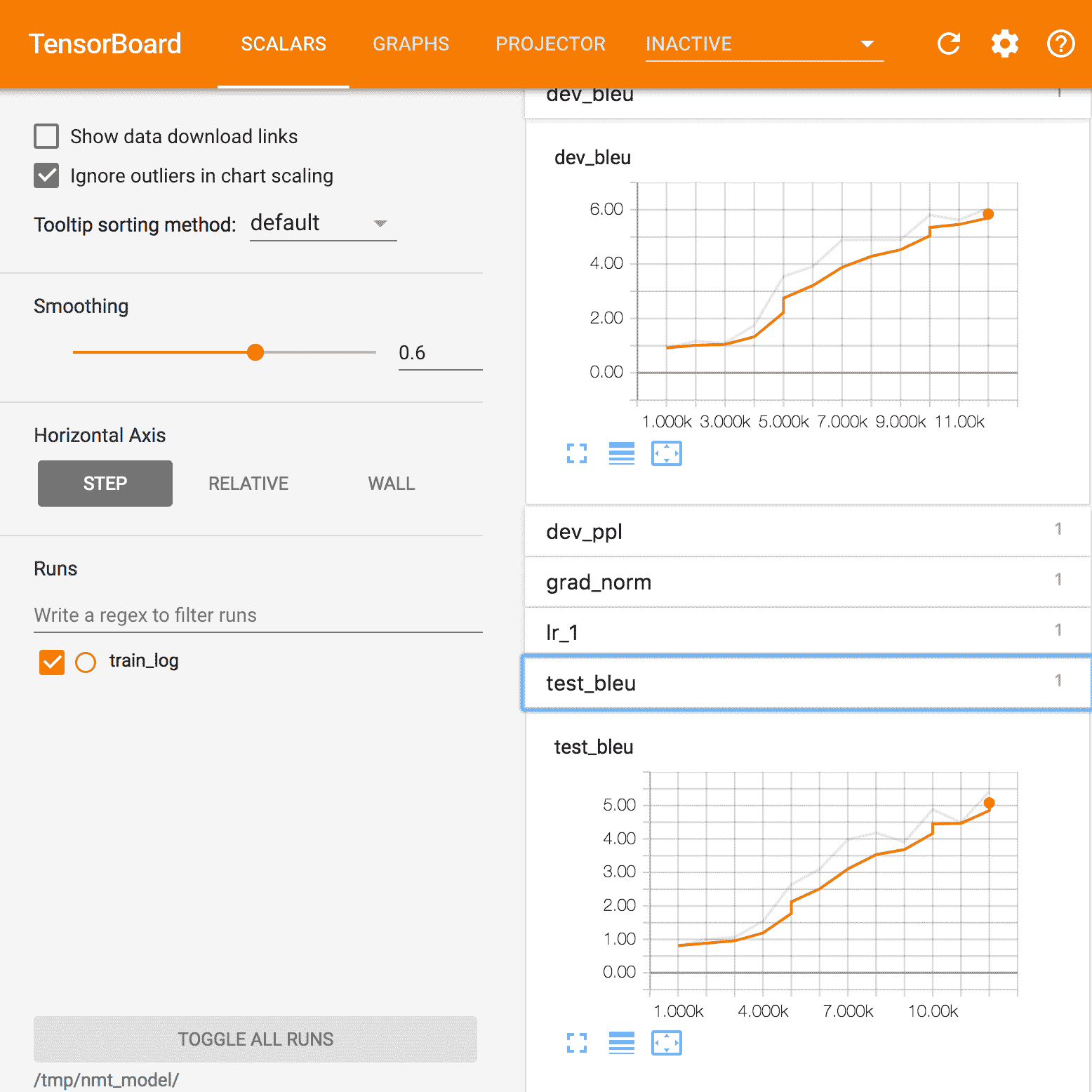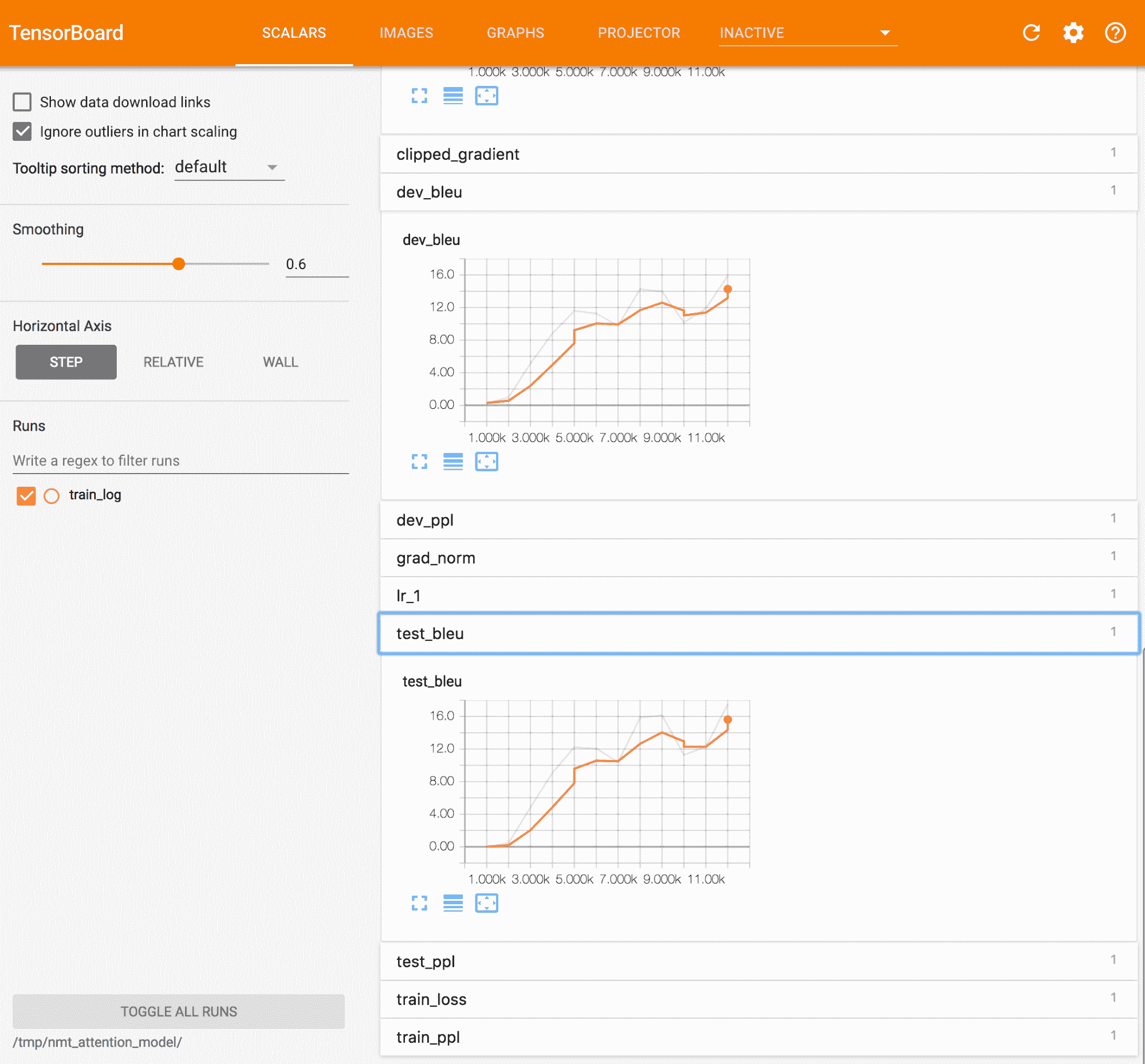 該代碼學習如何翻譯，并通過 BLEU 度量標準通過迭代跟蹤進度，如下圖所示：  Tensorboard 中的 BLEU 指標示例 # 神經機器翻譯 -- 用 seq2seq RNN 推理 在此秘籍中，我們使用先前秘籍的結果將源語言轉換為目標語言。 這個想法非常簡單：給源語句提供兩個組合的 RNN（編碼器+解碼器）作為輸入。 句子一結束，解碼器將產生對率值，我們*貪婪地*產生與最大值關聯的單詞。 例如，從解碼器產生單詞`moi`作為第一個令牌，因為該單詞具有最大對率值。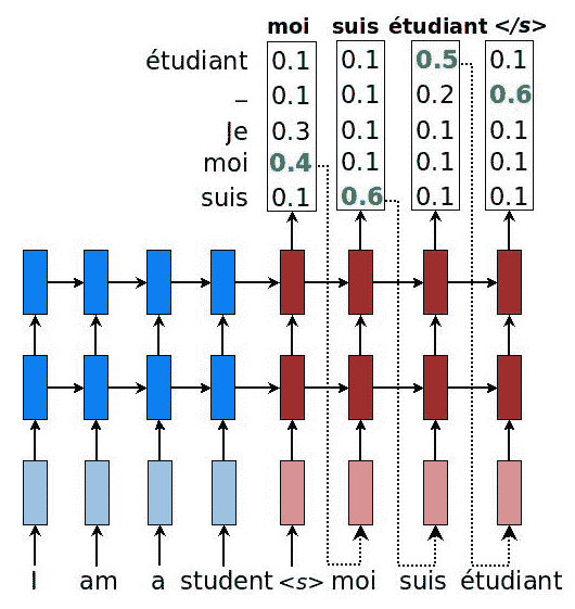 之后，會產生單詞`suis`，依此類推：  [具有概率的 NM 序列模型的示例](https://github.com/lmthang/thesis/blob/master/thesis.pdf) 使用解碼器的輸出有多種策略： * **貪婪**：產生對應最大對率的字 * **采樣**：通過對產生的對率進行采樣來產生單詞 * **集束搜索**：一個以上的預測，因此創建了可能的擴展樹 # 操作步驟 我們按以下步驟進行： 1. 定義用于對解碼器進行采樣的貪婪策略。 這很容易，因為我們可以使用`tf.contrib.seq2seq.GreedyEmbeddingHelper`中定義的庫。 由于我們不知道目標句子的確切長度，因此我們將啟發式方法限制為最大長度為源句子長度的兩倍： ```py # Helper helper = tf.contrib.seq2seq.GreedyEmbeddingHelper( embedding_decoder, tf.fill([batch_size], tgt_sos_id), tgt_eos_id) # Decoder decoder = tf.contrib.seq2seq.BasicDecoder( decoder_cell, helper, encoder_state, output_layer=projection_layer) # Dynamic decoding outputs, _ = tf.contrib.seq2seq.dynamic_decode( decoder, maximum_iterations=maximum_iterations) translations = outputs.sample_id maximum_iterations = tf.round(tf.reduce_max(source_sequence_length) * 2) ``` 2. 現在，我們可以運行網絡，輸入一個從未見過的句子（`inference_input_file=/tmp/my_infer_file`），然后讓網絡翻譯結果（`inference_output_file=/tmp/nmt_model/output_infer`）： ```py python -m nmt.nmt \ --out_dir=/tmp/nmt_model \ --inference_input_file=/tmp/my_infer_file.vi \ --inference_output_file=/tmp/nmt_model/output_infer ``` # 工作原理 將兩個 RNN *打包在一起*，以形成編碼器-解碼器 RNN 網絡。 解碼器產生對率，然后將其貪婪地轉換為目標語言的單詞。 例如，此處顯示了從越南語到英語的自動翻譯： * **用英語輸入的句子**：小時候，我認為朝鮮是世界上最好的國家，我經常唱歌&。 我們沒有什么可嫉妒的。 * **翻譯成英語的輸出句子**：當我非常好時，我將去了解最重要的事情，而我不確定該說些什么。 # 您只需要注意力 -- seq2seq RNN 的另一個示例 在本秘籍中，我們介紹了[**注意力**方法](https://arxiv.org/abs/1409.0473)（Dzmitry Bahdanau，Kyunghyun Cho 和 Yoshua Bengio，ICLR 2015），這是神經網絡翻譯的最新解決方案。 ，它包括在編碼器和解碼器 RNN 之間添加其他連接。 實際上，僅將解碼器與編碼器的最新層連接會帶來信息瓶頸，并且不一定允許通過先前的編碼器層獲取的信息通過。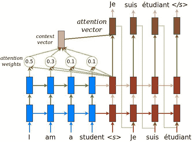 下圖說明了采用的解決方案：  [NMT 注意力模型的示例](https://github.com/lmthang/thesis/blob/master/thesis.pdf) 需要考慮三個方面： * 首先，將當前目標隱藏狀態與所有先前的源狀態一起使用以得出注意力權重，該注意力權重用于或多或少地關注序列中先前看到的標記 * 其次，創建上下文向量以匯總注意力權重的結果 * 第三，將上下文向量與當前目標隱藏狀態組合以獲得注意力向量 # 操作步驟 我們按以下步驟進行： 1. 使用庫`tf.contrib.seq2seq.LuongAttention`定義注意力機制，該庫實現了 Minh-Thang Luong，Hieu Pham 和 Christopher D. Manning（2015 年）在《基于注意力的神經機器翻譯有效方法》中定義的注意力模型： ```py # attention_states: [batch_size, max_time, num_units] attention_states = tf.transpose(encoder_outputs, [1, 0, 2]) # Create an attention mechanism attention_mechanism = tf.contrib.seq2seq.LuongAttention( num_units, attention_states, memory_sequence_length=source_sequence_length) ``` 2. 通過注意力包裝器，將定義的注意力機制用作解碼器單元周圍的包裝器： ```py decoder_cell = tf.contrib.seq2seq.AttentionWrapper( decoder_cell, attention_mechanism, attention_layer_size=num_units) ``` 3. 運行代碼以查看結果。 我們立即注意到，注意力機制在 BLEU 得分方面產生了顯著改善： ```py python -m nmt.nmt \ > --attention=scaled_luong \ > --src=vi --tgt=en \ > --vocab_prefix=/tmp/nmt_data/vocab \ > --train_prefix=/tmp/nmt_data/train \ > --dev_prefix=/tmp/nmt_data/tst2012 \ > --test_prefix=/tmp/nmt_data/tst2013 \ > --out_dir=/tmp/nmt_attention_model \ > --num_train_steps=12000 \ > --steps_per_stats=100 \ > --num_layers=2 \ > --num_units=128 \ > --dropout=0.2 \ > --metrics=bleu [...] # Start step 0, lr 1, Fri Sep 22 22:49:12 2017 # Init train iterator, skipping 0 elements global step 100 lr 1 step-time 1.71s wps 3.23K ppl 15193.44 bleu 0.00 [...] # Final, step 12000 lr 0.98 step-time 1.67 wps 3.37K ppl 14.64, dev ppl 14.01, dev bleu 15.9, test ppl 12.58, test bleu 17.5, Sat Sep 23 04:35:42 2017 # Done training!, time 20790s, Sat Sep 23 04:35:42 2017. # Start evaluating saved best models. [..] loaded infer model parameters from /tmp/nmt_attention_model/best_bleu/translate.ckpt-12000, time 0.06s # 608 src: nh?ng b?n bi?t ?i?u gì kh?ng ? ref: But you know what ? nmt: But what do you know ? [...] # Best bleu, step 12000 step-time 1.67 wps 3.37K, dev ppl 14.01, dev bleu 15.9, test ppl 12.58, test bleu 17.5, Sat Sep 23 04:36:35 2017 ``` # 工作原理 注意是一種機制，該機制使用由編碼器 RNN 的內部狀態獲取的信息，并將該信息與解碼器的最終狀態進行組合。 關鍵思想是，通過這種方式，有可能或多或少地關注源序列中的某些標記。 下圖顯示了 BLEU 得分，引起了關注。 我們注意到，相對于我們第一個秘籍中未使用任何注意力的圖表而言，它具有明顯的優勢：  Tensorboard 中注意力的 BLEU 指標示例 # 更多 值得記住的是 seq2seq 不僅可以用于機器翻譯。 讓我們看一些例子： * Lukasz Kaiser 在[作為外語的語法](https://arxiv.org/abs/1412.7449)中，使用 seq2seq 模型來構建選區解析器。 選區分析樹將文本分為多個子短語。 樹中的非終結符是短語的類型，終結符是句子中的單詞，并且邊緣未標記。 * seq2seq 的另一個應用是 SyntaxNet，又名 Parsey McParserFace（[語法分析器](https://research.googleblog.com/2016/05/announcing-syntaxnet-worlds-most.html)），它是許多 NLU 系統中的關鍵第一組件。 給定一個句子作為輸入，它將使用描述單詞的句法特征的**詞性**（**POS**）標簽標記每個單詞，并確定句子中單詞之間的句法關系，在依存關系分析樹中表示。 這些句法關系與所討論句子的潛在含義直接相關。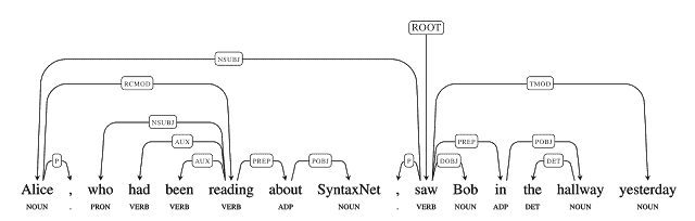 下圖使我們對該概念有了一個很好的了解：  [SyntaxNet 的一個例子](https://research.googleblog.com/2016/05/announcing-syntaxnet-worlds-most.html) # 通過 RNN 學習寫作莎士比亞 在本秘籍中，我們將學習如何生成與威廉·莎士比亞（William Shakespeare）相似的文本。 關鍵思想很簡單：我們將莎士比亞寫的真實文本作為輸入，并將其作為輸入 RNN 的輸入，該 RNN 將學習序列。 然后將這種學習用于生成新文本，該文本看起來像最偉大的作家用英語撰寫的文本。 為了簡單起見，我們將使用框架 [TFLearn](http://tflearn.org/)，它在 TensorFlow 上運行。 此示例是標準分發版的一部分，[可從以下位置獲得](https://github.com/tflearn/tflearn/blob/master/examples/nlp/lstm_generator_shakespeare.py)。開發的模型是 RNN 字符級語言模型，其中考慮的序列是字符序列而不是單詞序列。 # 操作步驟 我們按以下步驟進行： 1. 使用`pip`安裝 TFLearn： ```py pip install -I tflearn ``` 2. 導入許多有用的模塊并下載一個由莎士比亞撰寫的文本示例。 在這種情況下，我們使用[這個頁面](https://raw.githubusercontent.com/tflearn/tflearn.github.io/master/resources/shakespeare_input.txt)中提供的一種： ```py import os import pickle from six.moves import urllib import tflearn from tflearn.data_utils import * path = "shakespeare_input.txt" char_idx_file = 'char_idx.pickle' if not os.path.isfile(path): urllib.request.urlretrieve("https://raw.githubusercontent.com/tflearn/tflearn.github.io/master/resources/shakespeare_input.txt", path) ``` 3. 使用`string_to_semi_redundant_sequences()`將輸入的文本轉換為向量，并返回解析的序列和目標以及相關的字典，該函數將返回一個元組（輸入，目標，字典）： ```py maxlen = 25 char_idx = None if os.path.isfile(char_idx_file): print('Loading previous char_idx') char_idx = pickle.load(open(char_idx_file, 'rb')) X, Y, char_idx = \ textfile_to_semi_redundant_sequences(path, seq_maxlen=maxlen, redun_step=3, pre_defined_char_idx=char_idx) pickle.dump(char_idx, open(char_idx_file,'wb')) ``` 4. 定義一個由三個 LSTM 組成的 RNN，每個 LSTM 都有 512 個節點，并返回完整序列，而不是僅返回最后一個序列輸出。 請注意，我們使用掉線模塊連接 LSTM 模塊的可能性為 50%。 最后一層是密集層，其應用 softmax 的長度等于字典大小。 損失函數為`categorical_crossentropy`，優化器為 Adam： ```py g = tflearn.input_data([None, maxlen, len(char_idx)]) g = tflearn.lstm(g, 512, return_seq=True) g = tflearn.dropout(g, 0.5) g = tflearn.lstm(g, 512, return_seq=True) g = tflearn.dropout(g, 0.5) g = tflearn.lstm(g, 512) g = tflearn.dropout(g, 0.5) g = tflearn.fully_connected(g, len(char_idx), activation='softmax') g = tflearn.regression(g, optimizer='adam', loss='categorical_crossentropy', learning_rate=0.001) ``` 5. 給定步驟 4 中定義的網絡，我們現在可以使用庫`flearn.models.generator.SequenceGenerator`（`network`，`dictionary=char_idx, seq_maxlen=maxle`和`clip_gradients=5.0, checkpoint_path='model_shakespeare'`）生成序列： ```py m = tflearn.SequenceGenerator(g, dictionary=char_idx, seq_maxlen=maxlen, clip_gradients=5.0, checkpoint_path='model_shakespeare') ``` 6. 對于 50 次迭代，我們從輸入文本中獲取隨機序列，然后生成一個新文本。 溫度正在控制所創建序列的新穎性； 溫度接近 0 看起來像用于訓練的樣本，而溫度越高，新穎性越強： ```py for i in range(50): seed = random_sequence_from_textfile(path, maxlen) m.fit(X, Y, validation_set=0.1, batch_size=128, n_epoch=1, run_id='shakespeare') print("-- TESTING...") print("-- Test with temperature of 1.0 --") print(m.generate(600, temperature=1.0, seq_seed=seed)) print("-- Test with temperature of 0.5 --") print(m.generate(600, temperature=0.5, seq_seed=seed)) ``` # 工作原理 當新的未知或被遺忘的藝術品要歸功于作者時，有著名的學者將其與作者的其他作品進行比較。 學者們要做的是在著名作品的文本序列中找到共同的模式，希望在未知作品中找到相似的模式。 這種方法的工作方式相似：RNN 了解莎士比亞作品中最特殊的模式是什么，然后將這些模式用于生成新的，從未見過的文本，這些文本很好地代表了最偉大的英語作者的風格。 讓我們看一些執行示例： ```py python shakespeare.py Loading previous char_idx Vectorizing text... Text total length: 4,573,338 Distinct chars : 67 Total sequences : 1,524,438 --------------------------------- Run id: shakespeare Log directory: /tmp/tflearn_logs/ ``` # 第一次迭代 在這里，網絡正在學習一些基本結構，包括需要建立有關虛構字符（`DIA`，`SURYONT`，`HRNTLGIPRMAR`和`ARILEN`）的對話。 但是，英語仍然很差，很多單詞不是真正的英語： ```py --------------------------------- Training samples: 1371994 Validation samples: 152444 -- Training Step: 10719 | total loss: 2.22092 | time: 22082.057s | Adam | epoch: 001 | loss: 2.22092 | val_loss: 2.12443 -- iter: 1371994/1371994 -- TESTING... -- Test with temperature of 1.0 -- 'st thou, malice? If thou caseghough memet oud mame meard'ke. Afs weke wteak, Dy ny wold' as to of my tho gtroy ard has seve, hor then that wordith gole hie, succ, caight fom? DIA: A gruos ceen, I peey by my Wiouse rat Sebine would. waw-this afeean. SURYONT: Teeve nourterong a oultoncime bucice'is furtutun Ame my sorivass; a mut my peant? Am: Fe, that lercom ther the nome, me, paatuy corns wrazen meas ghomn'ge const pheale, As yered math thy vans: I im foat worepoug and thit mije woml! HRNTLGIPRMAR: I'd derfomquesf thiy of doed ilasghele hanckol, my corire-hougangle! Kiguw troll! you eelerd tham my fom Inow lith a -- Test with temperature of 0.5 -- 'st thou, malice? If thou prall sit I har, with and the sortafe the nothint of the fore the fir with with the ceme at the ind the couther hit yet of the sonsee in solles and that not of hear fore the hath bur. ARILEN: More you a to the mare me peod sore, And fore string the reouck and and fer to the so has the theat end the dore; of mall the sist he the bot courd wite be the thoule the to nenge ape and this not the the ball bool me the some that dears, The be to the thes the let the with the thear tould fame boors and not to not the deane fere the womour hit muth so thand the e meentt my to the treers and woth and wi ``` # 經過幾次迭代 在這里，網絡開始學習對話的正確結構，并且使用`Well, there shall the things to need the offer to our heart`和`There is not that be so then to the death To make the body and all the mind`這樣的句子，書面英語看起來更正確： ```py --------------------------------- Training samples: 1371994 Validation samples: 152444 -- Training Step: 64314 | total loss: 1.44823 | time: 21842.362s | Adam | epoch: 006 | loss: 1.44823 | val_loss: 1.40140 -- iter: 1371994/1371994 -- -- Test with temperature of 0.5 -- in this kind. THESEUS: There is not that be so then to the death To make the body and all the mind. BENEDICK: Well, there shall the things to need the offer to our heart, To not are he with him: I have see the hands are to true of him that I am not, The whom in some the fortunes, Which she were better not to do him? KING HENRY VI: I have some a starter, and and seen the more to be the boy, and be such a plock and love so say, and I will be his entire, And when my masters are a good virtues, That see the crown of our worse, This made a called grace to hear him and an ass, And the provest and stand, ``` # 更多 博客文章[循環神經網絡的不合理有效性](http://karpathy.github.io/2015/05/21/rnn-effectiveness/)描述了一組引人入勝的示例 RNN 字符級語言模型，包括以下內容： * 莎士比亞文本生成類似于此示例 * Wikipedia 文本生成類似于此示例，但是基于不同的訓練文本 * 代數幾何（LaTex）文本生成類似于此示例，但基于不同的訓練文本 * Linux 源代碼文本的生成與此示例相似，但是基于不同的訓練文本 * 嬰兒命名文本的生成與此示例類似，但是基于不同的訓練文本 # 學習使用 RNN 預測未來的比特幣價值 在本秘籍中，我們將學習如何使用 RNN 預測未來的比特幣價值。 關鍵思想是，過去觀察到的值的時間順序可以很好地預測未來的值。 對于此秘籍，我們將使用 MIT 許可下的[這個頁面](https://github.com/guillaume-chevalier/seq2seq-signal-prediction)上提供的代碼。 給定時間間隔的比特幣值通過 API 從[這里](https://www.coindesk.com/api/)下載。 這是 API 文檔的一部分： ```py We offer historical data from our Bitcoin Price Index through the following endpoint: https://api.coindesk.com/v1/bpi/historical/close.json By default, this will return the previous 31 days' worth of data. This endpoint accepts the following optional parameters: ?index=[USD/CNY]The index to return data for. Defaults to USD. ?currency=<VALUE>The currency to return the data in, specified in ISO 4217 format. Defaults to USD. ?start=<VALUE>&end=<VALUE> Allows data to be returned for a specific date range. Must be listed as a pair of start and end parameters, with dates supplied in the YYYY-MM-DD format, e.g. 2013-09-01 for September 1st, 2013. ?for=yesterday Specifying this will return a single value for the previous day. Overrides the start/end parameter. Sample Request: https://api.coindesk.com/v1/bpi/historical/close.json?start=2013-09-01&end=2013-09-05 Sample JSON Response: {"bpi":{"2013-09-01":128.2597,"2013-09-02":127.3648,"2013-09-03":127.5915,"2013-09-04":120.5738,"2013-09-05":120.5333},"disclaimer":"This data was produced from the CoinDesk Bitcoin Price Index. BPI value data returned as USD.","time":{"updated":"Sep 6, 2013 00:03:00 UTC","updatedISO":"2013-09-06T00:03:00+00:00"}} ``` # 操作步驟 這是我們進行秘籍的方法： 1. 克隆以下 GitHub 存儲庫。 這是一個鼓勵用戶嘗試使用 seq2seq 神經網絡架構的項目： ```py git clone https://github.com/guillaume-chevalier/seq2seq-signal-prediction.git ``` 2. 給定前面的存儲庫，請考慮以下函數，這些函數可加載和標準化 USD 或 EUR 比特幣值的比特幣歷史數據。 這些特征在`dataset.py`中定義。 訓練和測試數據根據 80/20 規則分開。 因此，測試數據的 20% 是最新的歷史比特幣值。 每個示例在特征軸/維度中包含 40 個 USD 數據點，然后包含 EUR 數據。 根據平均值和標準差對數據進行歸一化。 函數`generate_x_y_data_v4`生成大小為`batch_size`的訓練數據（分別是測試數據）的隨機樣本： ```py def loadCurrency(curr, window_size): """ Return the historical data for the USD or EUR bitcoin value. Is done with an web API call. curr = "USD" | "EUR" """ # For more info on the URL call, it is inspired by : # https://github.com/Levino/coindesk-api-node r = requests.get( "http://api.coindesk.com/v1/bpi/historical/close.json?start=2010-07-17&end=2017-03-03&currency={}".format( curr ) ) data = r.json() time_to_values = sorted(data["bpi"].items()) values = [val for key, val in time_to_values] kept_values = values[1000:] X = [] Y = [] for i in range(len(kept_values) - window_size * 2): X.append(kept_values[i:i + window_size]) Y.append(kept_values[i + window_size:i + window_size * 2]) # To be able to concat on inner dimension later on: X = np.expand_dims(X, axis=2) Y = np.expand_dims(Y, axis=2) return X, Y def normalize(X, Y=None): """ Normalise X and Y according to the mean and standard deviation of the X values only. """ # # It would be possible to normalize with last rather than mean, such as: # lasts = np.expand_dims(X[:, -1, :], axis=1) # assert (lasts[:, :] == X[:, -1, :]).all(), "{}, {}, {}. {}".format(lasts[:, :].shape, X[:, -1, :].shape, lasts[:, :], X[:, -1, :]) mean = np.expand_dims(np.average(X, axis=1) + 0.00001, axis=1) stddev = np.expand_dims(np.std(X, axis=1) + 0.00001, axis=1) # print (mean.shape, stddev.shape) # print (X.shape, Y.shape) X = X - mean X = X / (2.5 * stddev) if Y is not None: assert Y.shape == X.shape, (Y.shape, X.shape) Y = Y - mean Y = Y / (2.5 * stddev) return X, Y return X def fetch_batch_size_random(X, Y, batch_size): """ Returns randomly an aligned batch_size of X and Y among all examples. The external dimension of X and Y must be the batch size (eg: 1 column = 1 example). X and Y can be N-dimensional. """ assert X.shape == Y.shape, (X.shape, Y.shape) idxes = np.random.randint(X.shape[0], size=batch_size) X_out = np.array(X[idxes]).transpose((1, 0, 2)) Y_out = np.array(Y[idxes]).transpose((1, 0, 2)) return X_out, Y_out X_train = [] Y_train = [] X_test = [] Y_test = [] def generate_x_y_data_v4(isTrain, batch_size): """ Return financial data for the bitcoin. Features are USD and EUR, in the internal dimension. We normalize X and Y data according to the X only to not spoil the predictions we ask for. For every window (window or seq_length), Y is the prediction following X. Train and test data are separated according to the 80/20 rule. Therefore, the 20 percent of the test data are the most recent historical bitcoin values. Every example in X contains 40 points of USD and then EUR data in the feature axis/dimension. It is to be noted that the returned X and Y has the same shape and are in a tuple. """ # 40 pas values for encoder, 40 after for decoder's predictions. seq_length = 40 global Y_train global X_train global X_test global Y_test # First load, with memoization: if len(Y_test) == 0: # API call: X_usd, Y_usd = loadCurrency("USD", window_size=seq_length) X_eur, Y_eur = loadCurrency("EUR", window_size=seq_length) # All data, aligned: X = np.concatenate((X_usd, X_eur), axis=2) Y = np.concatenate((Y_usd, Y_eur), axis=2) X, Y = normalize(X, Y) # Split 80-20: X_train = X[:int(len(X) * 0.8)] Y_train = Y[:int(len(Y) * 0.8)] X_test = X[int(len(X) * 0.8):] Y_test = Y[int(len(Y) * 0.8):] if isTrain: return fetch_batch_size_random(X_train, Y_train, batch_size) else: return fetch_batch_size_random(X_test, Y_test, batch_size) ``` 3. 生成訓練，驗證和測試數據，并定義許多超參數，例如`batch_size`，`hidden_dim`（RNN 中隱藏的神經元的數量）和`layers_stacked_count`（棧式循環單元的數量）。 此外，定義一些參數以微調優化器，例如優化器的學習率，迭代次數，用于優化器模擬退火的`lr_decay`，優化器的動量以及避免過擬合的 L2 正則化。 請注意，GitHub 存儲庫具有默認的`batch_size = 5`和`nb_iters = 150`，但使用`batch_size = 1000`和`nb_iters = 100000`獲得了更好的結果： ```py from datasets import generate_x_y_data_v4 generate_x_y_data = generate_x_y_data_v4 import tensorflow as tf import numpy as np import matplotlib.pyplot as plt %matplotlib inline sample_x, sample_y = generate_x_y_data(isTrain=True, batch_size=3) print("Dimensions of the dataset for 3 X and 3 Y training examples : ") print(sample_x.shape) print(sample_y.shape) print("(seq_length, batch_size, output_dim)") print sample_x, sample_y # Internal neural network parameters seq_length = sample_x.shape[0] # Time series will have the same past and future (to be predicted) lenght. batch_size = 5 # Low value used for live demo purposes - 100 and 1000 would be possible too, crank that up! output_dim = input_dim = sample_x.shape[-1] # Output dimension (e.g.: multiple signals at once, tied in time) hidden_dim = 12 # Count of hidden neurons in the recurrent units. layers_stacked_count = 2 # Number of stacked recurrent cells, on the neural depth axis. # Optmizer: learning_rate = 0.007 # Small lr helps not to diverge during training. nb_iters = 150 # How many times we perform a training step (therefore how many times we show a batch). lr_decay = 0.92 # default: 0.9 . Simulated annealing. momentum = 0.5 # default: 0.0 . Momentum technique in weights update lambda_l2_reg = 0.003 # L2 regularization of weights - avoids overfitting ``` 4. 將網絡定義為由基本 GRU 單元組成的編碼器/解碼器。 該網絡由`layers_stacked_count=2` RNN 組成，我們將使用 TensorBoard 可視化該網絡。 請注意，`hidden_dim = 12`是循環單元中的隱藏神經元： ```py tf.nn.seq2seq = tf.contrib.legacy_seq2seq tf.nn.rnn_cell = tf.contrib.rnn tf.nn.rnn_cell.GRUCell = tf.contrib.rnn.GRUCell tf.reset_default_graph() # sess.close() sess = tf.InteractiveSession() with tf.variable_scope('Seq2seq'): # Encoder: inputs enc_inp = [ tf.placeholder(tf.float32, shape=(None, input_dim), name="inp_{}".format(t)) for t in range(seq_length) ] # Decoder: expected outputs expected_sparse_output = [ tf.placeholder(tf.float32, shape=(None, output_dim), name="expected_sparse_output_".format(t)) for t in range(seq_length) ] # Give a "GO" token to the decoder. # You might want to revise what is the appended value "+ enc_inp[:-1]". dec_inp = [ tf.zeros_like(enc_inp[0], dtype=np.float32, name="GO") ] + enc_inp[:-1] # Create a `layers_stacked_count` of stacked RNNs (GRU cells here). cells = [] for i in range(layers_stacked_count): with tf.variable_scope('RNN_{}'.format(i)): cells.append(tf.nn.rnn_cell.GRUCell(hidden_dim)) # cells.append(tf.nn.rnn_cell.BasicLSTMCell(...)) cell = tf.nn.rnn_cell.MultiRNNCell(cells) # For reshaping the input and output dimensions of the seq2seq RNN: w_in = tf.Variable(tf.random_normal([input_dim, hidden_dim])) b_in = tf.Variable(tf.random_normal([hidden_dim], mean=1.0)) w_out = tf.Variable(tf.random_normal([hidden_dim, output_dim])) b_out = tf.Variable(tf.random_normal([output_dim])) reshaped_inputs = [tf.nn.relu(tf.matmul(i, w_in) + b_in) for i in enc_inp] # Here, the encoder and the decoder uses the same cell, HOWEVER, # the weights aren't shared among the encoder and decoder, we have two # sets of weights created under the hood according to that function's def. dec_outputs, dec_memory = tf.nn.seq2seq.basic_rnn_seq2seq( enc_inp, dec_inp, cell ) output_scale_factor = tf.Variable(1.0, name="Output_ScaleFactor") # Final outputs: with linear rescaling similar to batch norm, # but without the "norm" part of batch normalization hehe. reshaped_outputs = [output_scale_factor*(tf.matmul(i, w_out) + b_out) for i in dec_outputs] # Merge all the summaries and write them out to /tmp/bitcoin_logs (by default) merged = tf.summary.merge_all() train_writer = tf.summary.FileWriter('/tmp/bitcoin_logs', sess.graph) ``` 5. 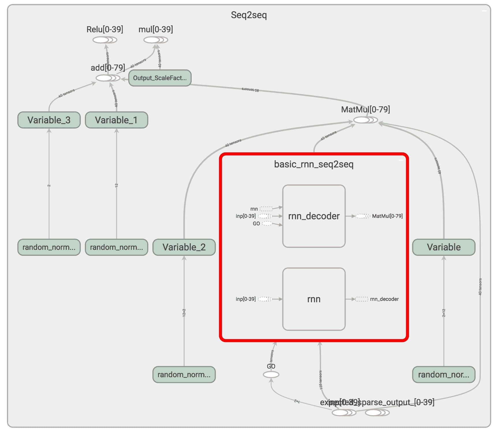現在讓我們運行 TensorBoard 并可視化由 RNN 編碼器和 RNN 解碼器組成的網絡： ```py tensorboard --logdir=/tmp/bitcoin_logs ``` 以下是代碼流程：  Tensorboard 中的比特幣價值預測代碼示例 6. 現在讓我們將損失函數定義為具有正則化的 L2 損失，以避免過擬合并獲得更好的泛化。 選擇的優化器是 RMSprop，其值為`learning_rate`，衰減和動量，如步驟 3 所定義： ```py # Training loss and optimizer with tf.variable_scope('Loss'): # L2 loss output_loss = 0 for _y, _Y in zip(reshaped_outputs, expected_sparse_output): output_loss += tf.reduce_mean(tf.nn.l2_loss(_y - _Y)) # L2 regularization (to avoid overfitting and to have a better generalization capacity) reg_loss = 0 for tf_var in tf.trainable_variables(): if not ("Bias" in tf_var.name or "Output_" in tf_var.name): reg_loss += tf.reduce_mean(tf.nn.l2_loss(tf_var)) loss = output_loss + lambda_l2_reg * reg_loss with tf.variable_scope('Optimizer'): optimizer = tf.train.RMSPropOptimizer(learning_rate, decay=lr_decay, momentum=momentum) train_op = optimizer.minimize(loss) ``` 7. 通過生成訓練數據并在數據集中的`batch_size`示例上運行優化器來為批量訓練做準備。 同樣，通過從數據集中的`batch_size`示例生成測試數據來準備測試。 訓練針對`nb_iters+1`迭代進行，每十個迭代中的一個用于測試結果： ```py def train_batch(batch_size): """ Training step that optimizes the weights provided some batch_size X and Y examples from the dataset. """ X, Y = generate_x_y_data(isTrain=True, batch_size=batch_size) feed_dict = {enc_inp[t]: X[t] for t in range(len(enc_inp))} feed_dict.update({expected_sparse_output[t]: Y[t] for t in range(len(expected_sparse_output))}) _, loss_t = sess.run([train_op, loss], feed_dict) return loss_t def test_batch(batch_size): """ Test step, does NOT optimizes. Weights are frozen by not doing sess.run on the train_op. """ X, Y = generate_x_y_data(isTrain=False, batch_size=batch_size) feed_dict = {enc_inp[t]: X[t] for t in range(len(enc_inp))} feed_dict.update({expected_sparse_output[t]: Y[t] for t in range(len(expected_sparse_output))}) loss_t = sess.run([loss], feed_dict) return loss_t[0] # Training train_losses = [] test_losses = [] sess.run(tf.global_variables_initializer()) for t in range(nb_iters+1): train_loss = train_batch(batch_size) train_losses.append(train_loss) if t % 10 == 0: # Tester test_loss = test_batch(batch_size) test_losses.append(test_loss) print("Step {}/{}, train loss: {}, \tTEST loss: {}".format(t, nb_iters, train_loss, test_loss)) print("Fin. train loss: {}, \tTEST loss: {}".format(train_loss, test_loss)) ``` 8. 可視化`n_predictions`結果。 我們將以黃色形象化`nb_predictions = 5`預測，以`x`形象化藍色的實際值`ix`。 請注意，預測從直方圖中的最后一個藍點開始，從視覺上，您可以觀察到，即使這個簡單的模型也相當準確： ```py # Test nb_predictions = 5 print("Let's visualize {} predictions with our signals:".format(nb_predictions)) X, Y = generate_x_y_data(isTrain=False, batch_size=nb_predictions) feed_dict = {enc_inp[t]: X[t] for t in range(seq_length)} outputs = np.array(sess.run([reshaped_outputs], feed_dict)[0]) for j in range(nb_predictions): plt.figure(figsize=(12, 3)) for k in range(output_dim): past = X[:,j,k] expected = Y[:,j,k] pred = outputs[:,j,k] label1 = "Seen (past) values" if k==0 else "_nolegend_" label2 = "True future values" if k==0 else "_nolegend_" label3 = "Predictions" if k==0 else "_nolegend_" plt.plot(range(len(past)), past, "o--b", label=label1) plt.plot(range(len(past), len(expected)+len(past)), expected, "x--b", label=label2) plt.plot(range(len(past), len(pred)+len(past)), pred, "o--y", label=label3) plt.legend(loc='best') plt.title("Predictions v.s. 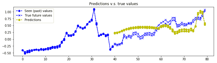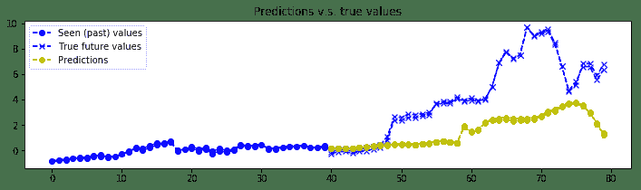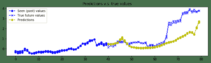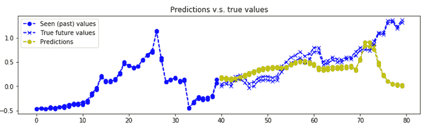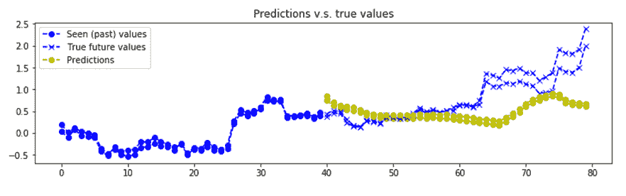true values") plt.show() ``` 我們得到的結果如下：      比特幣價值預測的一個例子 # 工作原理 帶有 GRU 基本單元的編碼器-解碼器層堆疊 RNN 用于預測比特幣值。 RNN 非常擅長學習序列，即使使用基于 2 層和 12 個 GRU 單元的簡單模型，比特幣的預測確實相當準確。 當然，此預測代碼并非鼓勵您投資比特幣，而只是討論深度學習方法。 而且，需要更多的實驗來驗證我們是否存在數據過擬合的情況。 # 更多 預測股市價值是一個不錯的 RNN 應用，并且有許多方便的包，例如： * Drnns-prediction 使用來自 Kaggle 的《股票市場每日新聞》數據集上的 Keras 神經網絡庫實現了深度 RNN。 數據集任務是使用當前和前一天的新聞頭條作為特征來預測 DJIA 的未來走勢。 開源代碼可從[這里](https://github.com/jvpoulos/drnns-prediction)獲得。 * 邁克爾·盧克（Michael Luk）撰寫了一篇有趣的博客文章，[內容涉及如何基于 RNN 預測可口可樂的庫存量](https://sflscientific.com/data-science-blog/2017/2/10/predicting-stock-volume-with-lstm)。 * Jakob Aungiers 寫了另一篇有趣的博客文章 [LSTM 神經網絡時間序列預測](http://www.jakob-aungiers.com/articles/a/LSTM-Neural-Network-for-Time-Series-Prediction)。 # 多對一和多對多 RNN 示例 在本秘籍中，我們通過提供 RNN 映射的各種示例來總結與 RNN 討論過的內容。 為了簡單起見，我們將采用 Keras 并演示如何編寫一對一，一對多，多對一和多對多映射，如下圖所示：  [RNN 序列的一個例子](http://karpathy.github.io/2015/05/21/rnn-effectiveness/) # 操作步驟 我們按以下步驟進行： 1. 如果要創建**一對一**映射，則這不是 RNN，而是密集層。 假設已經定義了一個模型，并且您想添加一個密集網絡。 然后可以在 Keras 中輕松實現： ```py model = Sequential() model.add(Dense(output_size, input_shape=input_shape)) ``` 2. 如果要創建**一對多**選項，可以使用`RepeatVector(...)`實現。 請注意，`return_sequences`是一個布爾值，用于決定是返回輸出序列中的最后一個輸出還是完整序列： ```py model = Sequential() model.add(RepeatVector(number_of_times,input_shape=input_shape)) model.add(LSTM(output_size, return_sequences=True)) ``` 3. 如果要創建**多對一**選項，則可以使用以下 LSTM 代碼段實現： ```py model = Sequential() model.add(LSTM(1, input_shape=(timesteps, data_dim))) ``` 4. 如果要創建**多對多**選項，當輸入和輸出的長度與循環步數匹配時，可以使用以下 LSTM 代碼段來實現： ```py model = Sequential() model.add(LSTM(1, input_shape=(timesteps, data_dim), return_sequences=True)) ``` # 工作原理 Keras 使您可以輕松編寫各種形狀的 RNN，包括一對一，一對多，多對一和多對多映射。 上面的示例說明了用 Keras 實現它們有多么容易。